Illustration of Ten Basic Algorithms in Artificial Intelligence

This article provides a general introduction to commonly used algorithms. It does not include code or complex theoretical derivations, but simply illustrates what these algorithms are and how they are applied.

Decision Tree

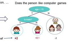
Classifies based on certain features by posing a question at each node, dividing the data into two categories, and continuing to ask questions. These questions are learned from existing data, and when new data is introduced, it can be classified into the appropriate leaves based on the questions on the tree.

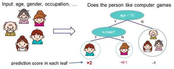
Figure 2: Illustration of the Decision Tree Principle

Random Forest

Randomly selects data from the source data to form several subsets:

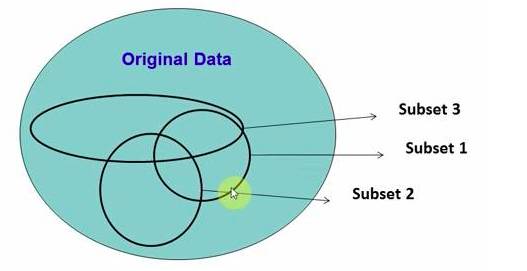
Figure 3-1: Illustration of the Random Forest Principle

S matrix is the source data, containing 1-N data points, A, B, C are features, and the last column C is the category:

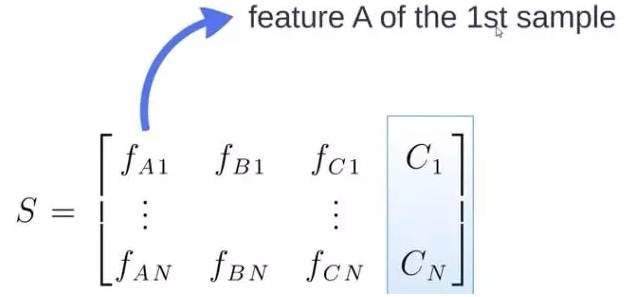
From S, randomly generate M submatrices:

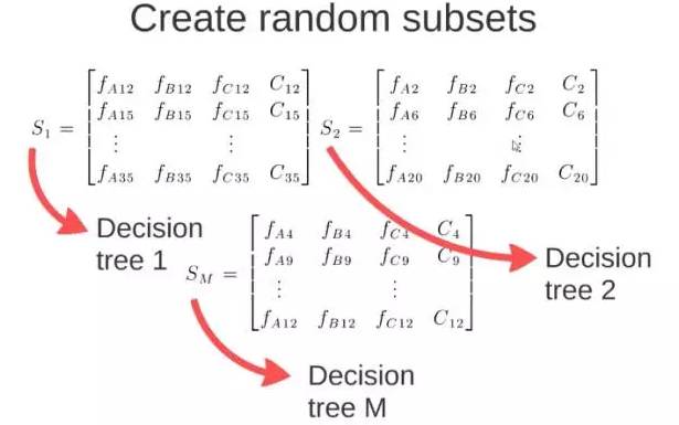
These M subsets produce M decision trees: New data is input into these M trees, resulting in M classification outcomes. The class with the highest count is taken as the final prediction result.

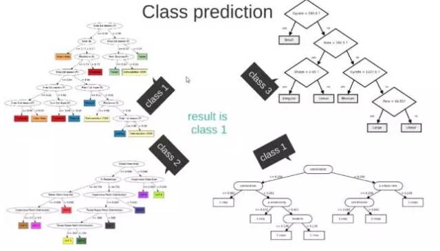
Figure 3-2: Random Forest Effect Demonstration

Logistic Regression

When the prediction target is a probability, the value range needs to satisfy being greater than or equal to 0 and less than or equal to 1. In this case, a simple linear model cannot achieve this, as the value will exceed the specified range when the domain is outside a certain range.

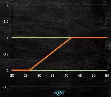
Figure 4-1: Linear Model Diagram

Thus, a model of such a shape is preferable:

Figure 4-2

How can such a model be obtained?

This model needs to satisfy two conditions: “greater than or equal to 0” and “less than or equal to 1”. The model that is greater than or equal to 0 can choose absolute values or square values; here we use the exponential function, which is always greater than 0. For being less than or equal to 1, we use division, where the numerator is itself and the denominator is itself plus 1, which ensures it is less than 1.

Figure 4-3

After some transformation, we obtain the logistic regression model:

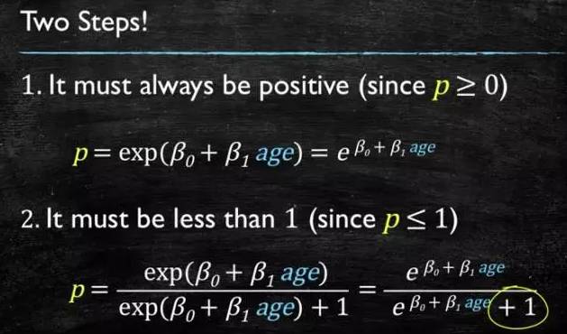
Figure 4-4

By calculating from the source data, we can obtain the corresponding coefficients:

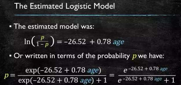
Figure 4-5

Finally, we obtain the figure of logistic:

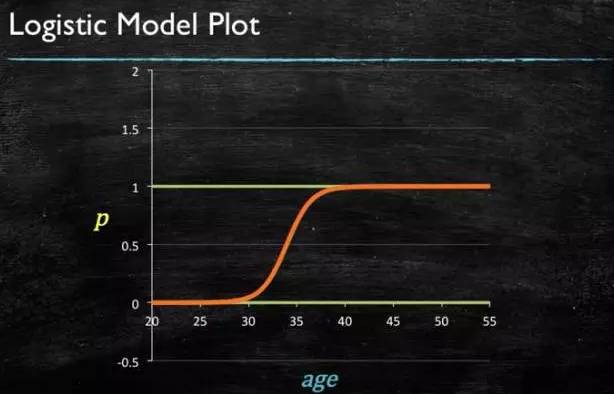
Figure 4-6: LR Model Curve

Support Vector Machine

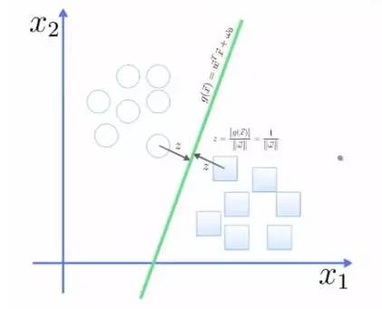
To separate two classes, we want to obtain a hyperplane, where the optimal hyperplane maximizes the margin to both classes. The margin is the distance from the hyperplane to the closest point, as shown in the figure, Z2>Z1, so the green hyperplane is better.

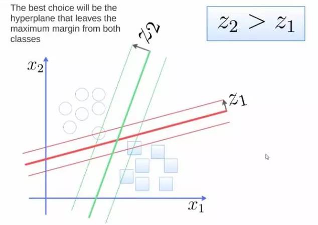
Figure 5: Classification Problem Illustration

We express this hyperplane as a linear equation, where one class is greater than or equal to 1 and the other class is less than or equal to -1:

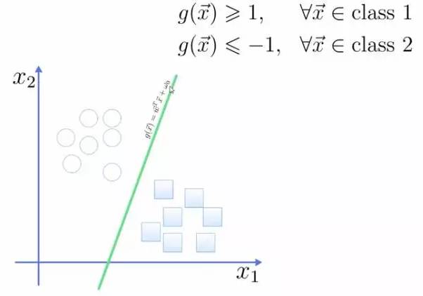
The distance from the point to the plane is calculated using the formula in the figure:

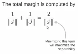
Thus, the expression for the total margin is as follows. The goal is to maximize this margin, which requires minimizing the denominator, turning it into an optimization problem:

For example, with three points, find the optimal hyperplane defined by the weight vector = (2,3) – (1,1):

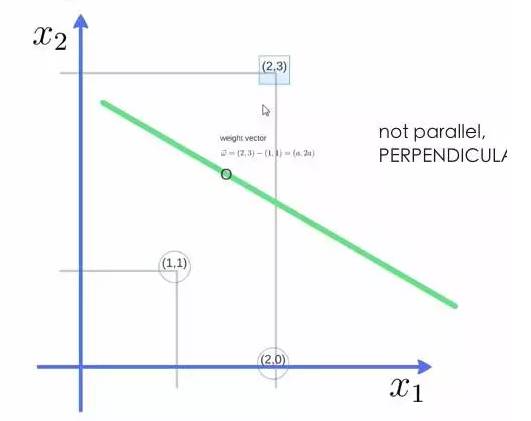
The weight vector obtained is (a, 2a). Substitute the two points into the equation, substituting (2,3) gives a value = 1, substituting (1,1) gives a value = -1, solving for a and the intercept w0 gives the expression for the hyperplane.

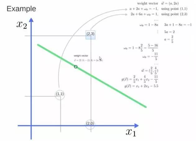
After solving for a, substituting (a, 2a) gives the support vector, and substituting a and w0 into the hyperplane equation gives the support vector machine.

Naive Bayes

For example, in NLP applications: Given a piece of text, return the sentiment classification, whether the attitude of this text is positive or negative:

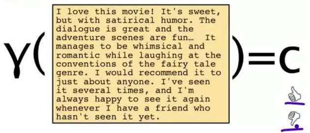
Figure 6-1: Problem Case

To solve this problem, we can focus on some of the words:

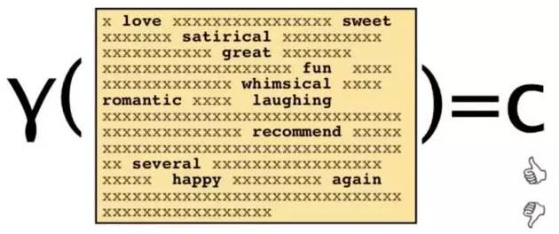
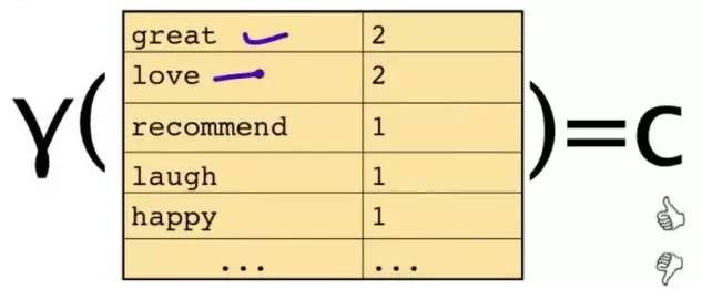
This text is represented by some words and their counts:

The original problem is: Given a sentence, which category does it belong to? By using Bayes’ rules, it becomes a simpler problem:

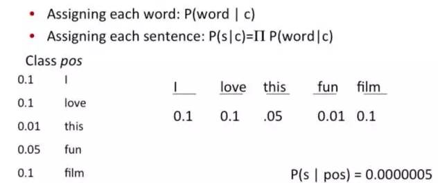
The problem becomes: What is the probability of this sentence appearing in this category? Of course, don’t forget the other two probabilities in the formula. For example, the probability of the word “love” appearing in a positive context is 0.1, and in a negative context it is 0.001.

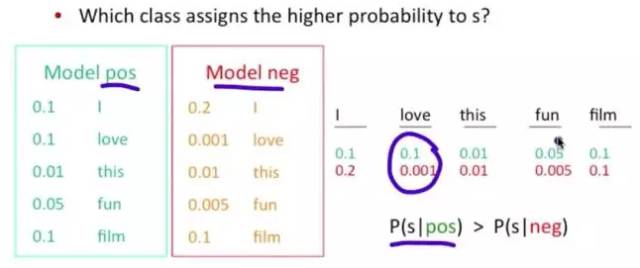
Figure 6-2: NB Algorithm Result Demonstration

K-Nearest Neighbors Algorithm

When given a new data point, it belongs to the class that is most common among the k nearest points.

Example: To distinguish between “cats” and “dogs”, if we use “claws” and “sound” as features, and the circles and triangles are known classifications, then which class does this “star” belong to?

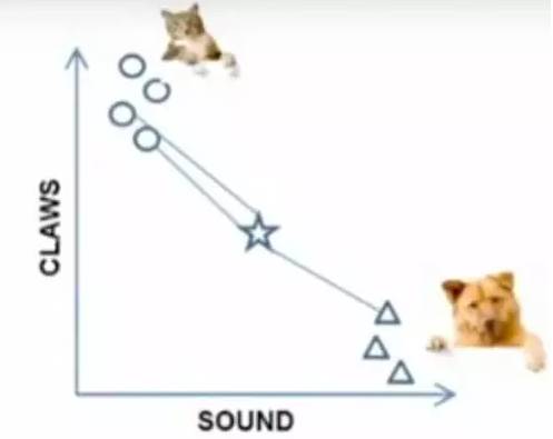
Figure 7-1: Problem Case

When k=3, the three points connected by these lines are the nearest three points. Since there are more circles, this star belongs to the category of cats.

Figure 7-2: Algorithm Steps Demonstration

K-Means Algorithm

First, a set of data is divided into three categories: pink has a high value, yellow has a low value. Initially, the simplest values 3, 2, 1 are chosen as the starting points for each category. The remaining data is then classified into the category of the nearest initial value.

Figure 8-1: Problem Case

After classification, the average value of each category is calculated as the new central point for the next round:

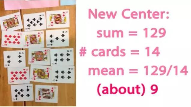
Figure 8-2

After several rounds, if the grouping no longer changes, the process can be stopped:

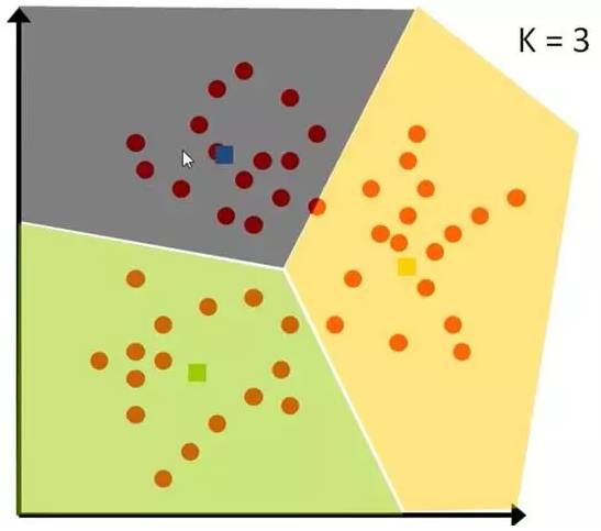
Figure 8-3: Algorithm Result Demonstration

Adaboost

Adaboost is one of the methods of Boosting. Boosting combines several classifiers that do not perform well individually to create a classifier that performs better collectively.

In the figure below, the two decision trees on the left and right do not perform well individually, but when the same data is input, considering both results increases their credibility.

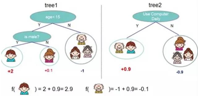
Figure 9-1: Algorithm Principle Demonstration

In an example of Adaboost, in handwritten recognition, many features can be captured on the drawing board, such as the direction of the starting point, the distance from the starting point to the ending point, etc.

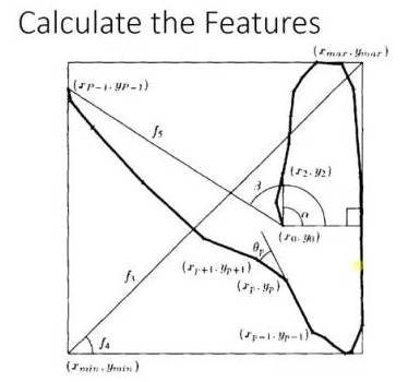
Figure 9-2

During training, the weight of each feature is obtained, for example, the starting parts of 2 and 3 are very similar, so this feature has little impact on classification, and its weight will be small.

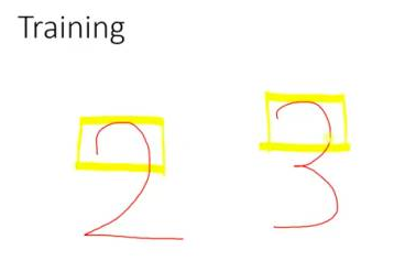
Figure 9-3

The angle alpha has strong recognition capability, so this feature will have a larger weight, and the final prediction result considers the results of these features.

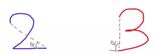
Figure 9-4

Neural Networks

Neural Networks are suitable for cases where an input may fall into at least two categories: NN consists of several layers of neurons and the connections between them. The first layer is the input layer, and the last layer is the output layer. Both the hidden layer and output layer have their own classifiers.

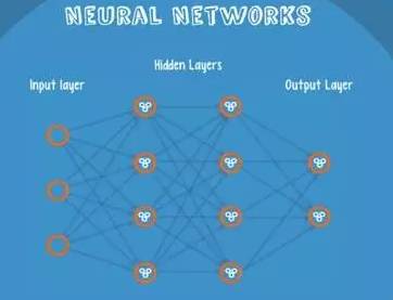
Figure 10-1: Neural Network Structure

The input is fed into the network, activated, and the computed scores are passed to the next layer. The activated neurons in the subsequent layers ultimately produce scores at the output layer representing the scores for various classes. In the example below, the classification result is class 1. The same input is transmitted to different nodes, resulting in different outcomes due to different weights and biases at each node, which is known as forward propagation.

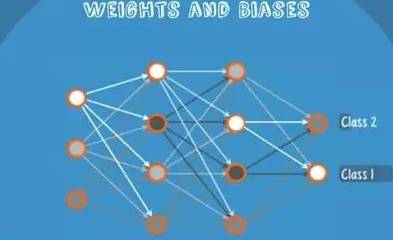
Figure 10-2: Algorithm Result Demonstration

Markov

Markov Chains consist of states and transitions. For example, based on the sentence ‘the quick brown fox jumps over the lazy dog’, we want to obtain Markov chains.

The steps involve first defining each word as a state and then calculating the probability of transitions between states.

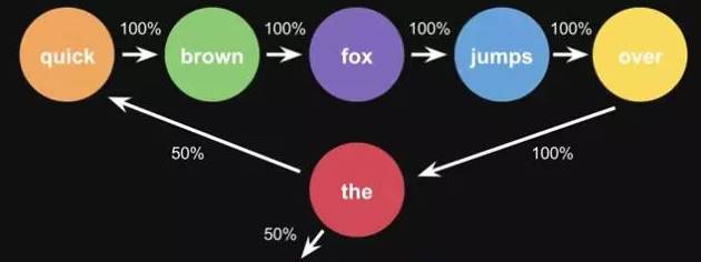
Figure 11-1: Markov Principle Illustration

This is the probability calculated from one sentence. When you use a large amount of text for statistics, you will obtain a larger state transition matrix, for example, the words that can follow ‘the’ and their corresponding probabilities.

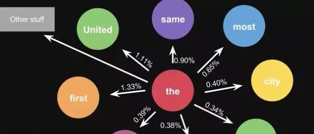
Figure 11-2: Algorithm Result

The ten types of machine learning algorithms mentioned above are practitioners of artificial intelligence development, and even today, they are still widely used in data mining and small sample artificial intelligence problems.

Source: Mathematical China WeChat Official Account