With the increasing popularity of Artificial Intelligence (AI) technology, various algorithms play a key role in driving the development of this field. From linear regression predicting housing prices to neural networks powering self-driving cars, these algorithms silently support the operation of countless applications.
Today, we will give you a glimpse of these popular AI algorithms (Linear Regression, Logistic Regression, Decision Trees, Naive Bayes, Support Vector Machines (SVM), Ensemble Learning, K-Nearest Neighbors, K-Means, Neural Networks, Deep Q-Networks), exploring their working principles, application scenarios, and their impact in the real world.
Model Principle: Linear regression attempts to find the best-fitting line that can approximate the data points in a scatter plot.
Model Training: The model is trained using known input and output data by minimizing the squared error between predicted and actual values.
Advantages: Simple and easy to understand, high computational efficiency.
Disadvantages: Limited ability to handle non-linear relationships.
Use Cases: Suitable for predicting continuous values, such as housing prices and stock prices.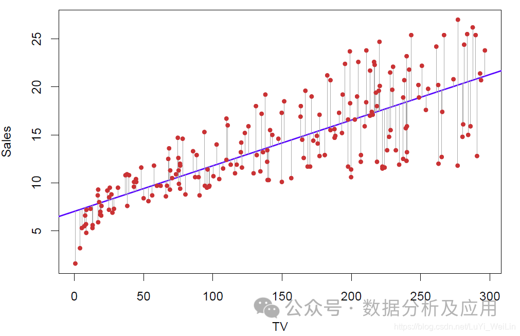 Example Code (Building a Simple Linear Regression Model Using Python’s Scikit-learn Library):
from sklearn.linear_model import LinearRegression
from sklearn.datasets import make_regression


# Generate simulated dataset
X, y = make_regression(n_samples=100, n_features=1, noise=0.1)


# Create linear regression model object
lr = LinearRegression()


# Train model
lr.fit(X, y)


# Make predictions
predictions = lr.predict(X)
Model Principle: Logistic regression is a machine learning algorithm used to solve binary classification problems. It maps continuous inputs to discrete outputs (usually binary). It uses a logistic function to map the results of linear regression to the (0,1) range, thus obtaining the probability of classification.
Model Training: The logistic regression model is trained using labeled sample data, optimizing the model’s parameters to minimize the cross-entropy loss between predicted probabilities and actual classifications.
Advantages: Simple and easy to understand, performs well on binary classification problems.
Disadvantages: Limited ability to handle non-linear relationships.
Use Cases: Suitable for binary classification problems, such as spam filtering and disease prediction.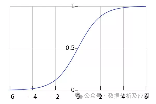 Example Code (Building a Simple Logistic Regression Model Using Python’s Scikit-learn Library):
from sklearn.linear_model import LogisticRegression
from sklearn.datasets import make_classification


# Generate simulated dataset
X, y = make_classification(n_samples=100, n_features=2, n_informative=2, n_redundant=0, random_state=42)


# Create logistic regression model object
lr = LogisticRegression()


# Train model
lr.fit(X, y)


# Make predictions
predictions = lr.predict(X)
Model Principle: Decision trees are a supervised learning algorithm that constructs decision boundaries by recursively partitioning the dataset into smaller subsets. Each internal node represents a judgment condition on a feature attribute, each branch represents a possible attribute value, and each leaf node represents a category.
Model Training: The decision tree is constructed by selecting the optimal partition attribute and using pruning techniques to prevent overfitting.
Advantages: Easy to understand and interpret, capable of handling both classification and regression problems.
Disadvantages: Prone to overfitting, sensitive to noise and outliers.
Use Cases: Suitable for classification and regression problems, such as credit card fraud detection and weather forecasting. Example Code (Building a Simple Decision Tree Model Using Python’s Scikit-learn Library):
from sklearn.tree import DecisionTreeClassifier
from sklearn.datasets import load_iris
from sklearn.model_selection import train_test_split


# Load dataset
iris = load_iris()
X = iris.data
y = iris.target


# Split into training and testing sets
X_train, X_test, y_train, y_test = train_test_split(X, y, test_size=0.2, random_state=42)


# Create decision tree model object
dt = DecisionTreeClassifier()


# Train model
dt.fit(X_train, y_train)


# Make predictions
predictions = dt.predict(X_test)
Model Principle: Naive Bayes is a classification method based on Bayes’ theorem and the assumption of feature conditional independence. It models the attribute values of samples in each category probabilistically and predicts the category of new samples based on these probabilities.
Model Training: It estimates the prior probabilities of each category and the conditional probabilities of each attribute using sample data with known categories and attributes to construct a Naive Bayes classifier.
Advantages: Simple, efficient, particularly effective for large categories and small datasets.
Disadvantages: Poor modeling of dependencies between features.
Use Cases: Suitable for text classification, spam filtering, etc.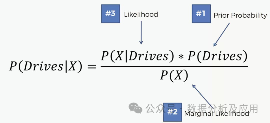 Example Code (Building a Simple Naive Bayes Classifier Using Python’s Scikit-learn Library):
from sklearn.naive_bayes import GaussianNB
from sklearn.datasets import load_iris


# Load dataset
iris = load_iris()
X = iris.data
y = iris.target


# Create Naive Bayes classifier object
gnb = GaussianNB()


# Train model
gnb.fit(X, y)


# Make predictions
predictions = gnb.predict(X)
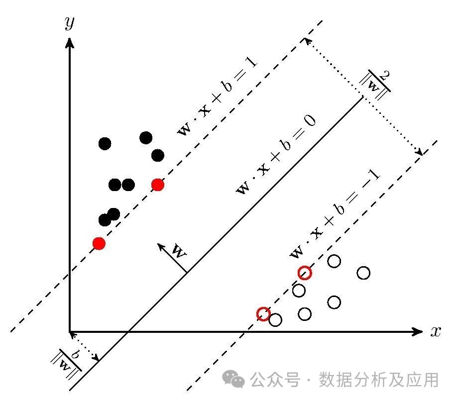
5. Support Vector Machines (SVM):
Model Principle: Support Vector Machines are a supervised learning algorithm used for classification and regression problems. It attempts to find a hyperplane that can separate samples of different categories. SVM uses kernel functions to handle non-linear problems.
Model Training: The SVM is trained by optimizing a quadratic loss function under constraints to find the optimal hyperplane.
Advantages: Performs well on high-dimensional data and non-linear problems, capable of handling multi-class problems.
Disadvantages: High computational complexity for large datasets, sensitive to parameter and kernel function selection.
Use Cases: Suitable for classification and regression problems, such as image recognition and text classification.
 Example Code (Building a Simple SVM Classifier Using Python’s Scikit-learn Library):
from sklearn import svm
from sklearn.datasets import load_iris
from sklearn.model_selection import train_test_split


# Load dataset
iris = load_iris()
X = iris.data
y = iris.target


# Split into training and testing sets
X_train, X_test, y_train, y_test = train_test_split(X, y, test_size=0.2, random_state=42)


# Create SVM classifier object using Radial Basis Function (RBF) kernel
clf = svm.SVC(kernel='rbf')


# Train model
clf.fit(X_train, y_train)


# Make predictions
predictions = clf.predict(X_test)
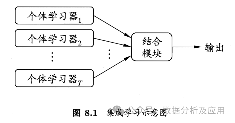
Model Principle: Ensemble learning is a method that improves prediction performance by constructing multiple base models and combining their predictions. Ensemble learning strategies include voting, averaging, stacking, and gradient boosting. Common ensemble learning models include XGBoost, Random Forest, and Adaboost.
Model Training: First, multiple base models are trained using the training dataset, and then their predictions are combined in some way to form the final prediction.
Advantages: Can improve the model’s generalization ability and reduce the risk of overfitting.
Disadvantages: High computational complexity, requiring more storage space and computational resources.
Use Cases: Suitable for solving classification and regression problems, especially for large datasets and complex tasks.
Example Code (Building a Simple Voting Ensemble Classifier Using Python’s Scikit-learn Library):
from sklearn.ensemble import VotingClassifier
from sklearn.linear_model import LogisticRegression
from sklearn.tree import DecisionTreeClassifier
from sklearn.datasets import load_iris
from sklearn.model_selection import train_test_split


# Load dataset
iris = load_iris()
X = iris.data
y = iris.target


# Split into training and testing sets
X_train, X_test, y_train, y_test = train_test_split(X, y, test_size=0.2, random_state=42)


# Create base model objects and ensemble classifier object
lr = LogisticRegression()
dt = DecisionTreeClassifier()
vc = VotingClassifier(estimators=[('lr', lr), ('dt', dt)], voting='hard')


# Train ensemble classifier
vc.fit(X_train, y_train)


# Make predictions
predictions = vc.predict(X_test)
Model Principle: K-Nearest Neighbors is an instance-based learning algorithm that predicts the category of a new sample by comparing it with known samples, finding the K closest samples, and voting based on their categories.
Model Training: No training phase is required; it finds the nearest neighbors by calculating the distance or similarity between the new sample and known samples.
Advantages: Simple, easy to understand, no training phase required.
Disadvantages: High computational complexity for large datasets, sensitive to the choice of parameter K.
Use Cases: Suitable for solving classification and regression problems, suitable for similarity measurement and classification tasks.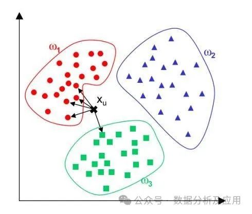 Example Code (Building a Simple K-Nearest Neighbor Classifier Using Python’s Scikit-learn Library):
from sklearn.neighbors import KNeighborsClassifier
from sklearn.datasets import load_iris
from sklearn.model_selection import train_test_split


# Load dataset
iris = load_iris()
X = iris.data
y = iris.target


# Split into training and testing sets
X_train, X_test, y_train, y_test = train_test_split(X, y, test_size=0.2, random_state=42)


# Create K-Nearest Neighbor classifier object, K=3
knn = KNeighborsClassifier(n_neighbors=3)


# Train model
knn.fit(X_train, y_train)


# Make predictions
predictions = knn.predict(X_test)
Model Principle: K-Means is an unsupervised learning algorithm used for clustering problems. It partitions n points (which can be sample data points) into k clusters so that each point belongs to the cluster corresponding to the nearest mean (cluster center).
Model Training: Clustering is achieved by iteratively updating the cluster centers and assigning each point to the nearest cluster center.
Advantages: Simple, fast, and performs well on large datasets.
Disadvantages: Sensitive to the initial cluster centers and may get stuck in local optima.
Use Cases: Suitable for clustering problems, such as market segmentation and anomaly detection.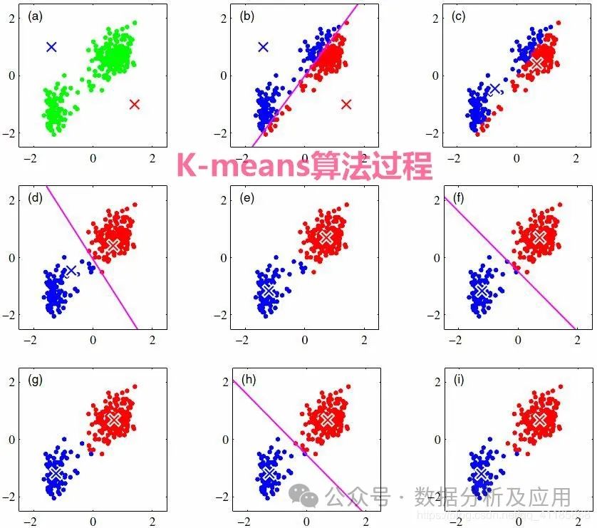 Example Code (Building a Simple K-Means Clustering Model Using Python’s Scikit-learn Library):
from sklearn.cluster import KMeans
from sklearn.datasets import make_blobs
import matplotlib.pyplot as plt


# Generate simulated dataset
X, y = make_blobs(n_samples=300, centers=4, cluster_std=0.60, random_state=0)


# Create K-Means clustering model object, K=4
kmeans = KMeans(n_clusters=4)


# Train model
kmeans.fit(X)


# Make predictions and get cluster labels
labels = kmeans.predict(X)


# Visualize results
plt.scatter(X[:, 0], X[:, 1], c=labels, cmap='viridis')
plt.show()
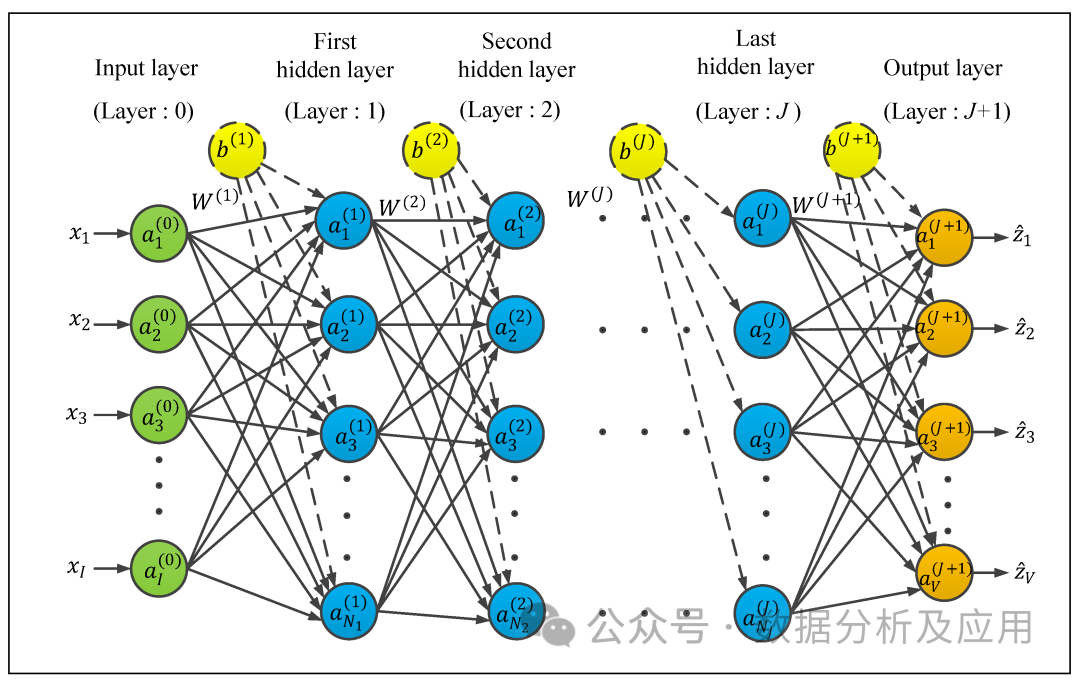
Model Principle: Neural networks are computational models that simulate the structure of human brain neurons, achieving complex pattern recognition and classification functions by simulating the input, output, and weight adjustment mechanisms of neurons. Neural networks consist of multiple layers of neurons, where the input layer receives external signals, and the output layer outputs results after processing through various layers of neurons.
Model Training: The training of neural networks is achieved through the backpropagation algorithm. During training, based on the error between the output result and the actual result, the error is backpropagated layer by layer, updating the weights and biases of the neurons to reduce the error.
Advantages: Capable of handling non-linear problems, possesses strong pattern recognition capabilities, and can learn complex patterns from large datasets.
Disadvantages: Prone to local optima, serious overfitting issues, long training time, and requires a large amount of data and computational resources.
Use Cases: Suitable for image recognition, speech recognition, natural language processing, recommendation systems, etc.
Example Code (Building a Simple Neural Network Classifier Using Python’s TensorFlow Library):
import tensorflow as tf
from tensorflow.keras import layers, models
from tensorflow.keras.datasets import mnist


# Load MNIST dataset
(x_train, y_train), (x_test, y_test) = mnist.load_data()


# Normalize input data
x_train = x_train / 255.0
x_test = x_test / 255.0


# Build neural network model
model = models.Sequential()
model.add(layers.Flatten(input_shape=(28, 28)))
model.add(layers.Dense(128, activation='relu'))
model.add(layers.Dense(10, activation='softmax'))


# Compile model and set loss function and optimizer parameters
model.compile(optimizer='adam', loss='sparse_categorical_crossentropy', metrics=['accuracy'])


# Train model
model.fit(x_train, y_train, epochs=5)


# Make predictions
predictions = model.predict(x_test)
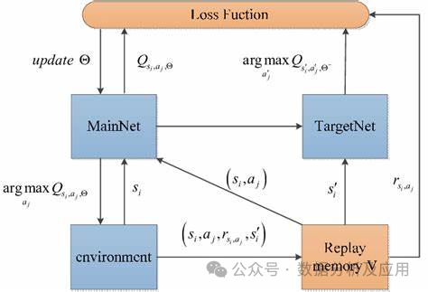
Deep Reinforcement Learning (DQN):
Model Principle: Deep Q-Networks (DQN) is a reinforcement learning algorithm that combines deep learning with Q-learning. Its core idea is to use a neural network to approximate the Q-function, i.e., the state-action value function, providing a basis for the agent to choose the optimal action in a given state.
Model Training: The training process of DQN includes two stages: offline and online. In the offline stage, the agent collects data through interaction with the environment and trains the neural network. In the online stage, the agent uses the neural network for action selection and updates. To address the overestimation problem, DQN introduces the concept of target networks, improving stability by keeping the target network stable for a period.
Advantages: Capable of handling high-dimensional state and action spaces, suitable for problems with continuous action spaces, and offers good stability and generalization capabilities.
Disadvantages: Prone to local optima, requires a large amount of data and computational resources, and is sensitive to parameter selection.
Use Cases: Suitable for scenarios such as gaming and robot control.
Example Code (Building a Simple DQN Reinforcement Learning Model Using Python’s TensorFlow Library):
import tensorflow as tf
from tensorflow.keras.models import Sequential
from tensorflow.keras.layers import Dense, Dropout, Flatten
from tensorflow.keras.optimizers import Adam
from tensorflow.keras import backend as K


class DQN:
def __init__(self, state_size, action_size):
self.state_size = state_size
self.action_size = action_size
self.memory = deque(maxlen=2000)
self.gamma = 0.85
self.epsilon = 1.0
self.epsilon_min = 0.01
self.epsilon_decay = 0.995
self.learning_rate = 0.005
self.model = self.create_model()
self.target_model = self.create_model()
self.target_model.set_weights(self.model.get_weights())


def create_model(self):
model = Sequential()
model.add(Flatten(input_shape=(self.state_size,)))
model.add(Dense(24, activation='relu'))
model.add(Dense(24, activation='relu'))
model.add(Dense(self.action_size, activation='linear'))
return model


def remember(self, state, action, reward, next_state, done):
self.memory.append((state, action, reward, next_state, done))


def act(self, state):
if len(self.memory) > 1000:
self.epsilon *= self.epsilon_decay
if self.epsilon < self.epsilon_min:
self.epsilon = self.epsilon_min
if np.random.rand() <= self.epsilon:
return random.randrange(self.action_size)
return np.argmax(self.model.predict(state)[0])