Click on the above “Beginner’s Guide to Vision” to select and add Star or Pin.

Important content delivered in real-time

This article is translated from: [Illustrated: Efficient Neural Architecture Search]

https://towardsdatascience.com/illustrated-efficient-neural-architecture-search-5f7387f9fb6 (Requires VPN)

• Reinforcement Learning

1. Neural Architecture Search with Reinforcement Learning [1]

2. Learning Transferable Architectures for Scalable Image Recognition [2]

3. Efficient Neural Architecture Search via Parameter Sharing [3]

• Genetic Algorithms

1. Hierarchical Representations for Efficient Architecture Search [4]

2. Regularized Evolution for Image Classifier Architecture Search [5]

• Sequential Model-Based Optimization

1. Progressive Neural Architecture Search [6]

• Bayesian Optimization

1. Auto-Keras: An Efficient Neural Architecture Search System [7]

2. Neural Architecture Search with Bayesian Optimisation and Optimal Transport [8]

• Gradient-Based Optimization

1. SNAS: Stochastic Neural Architecture Search [9]

2. DARTS: Differentiable Architecture Search [10]

Here, we mainly introduce Efficient Neural Architecture Search via Parameter Sharing (ENAS), a method that uses reinforcement learning to construct convolutional and recurrent neural networks. The authors propose a predefined neural network that is guided to generate new neural networks using a reinforcement learning framework with macro and micro search.

Table of Contents

• Overview

• Search Strategy

• Notes

• Conclusion

Overview

ENAS consists of two types of neural networks:

• Controller – A predefined recurrent neural network (RNN), typically a Long Short-Term Memory (LSTM) network

• Sub-model – A convolutional neural network (CNN) required for image classification tasks

Like most NAS algorithms, ENAS includes three aspects:

1. Search Space – All possible different structures or sub-models that can be generated

2. Search Strategy – The methods for generating these structures or sub-models

3. Performance Evaluation – The methods for measuring the effectiveness of the generated sub-models

Let’s see how these five concepts constitute ENAS.

The Controller generates a set of instructions (or more strictly, makes and selects decisions) using the Search Strategy to control or directly construct the structure of the sub-model. These decisions involve various types of operations that make up specific layers in the sub-model (such as convolution, pooling, etc.). Through these decisions, a sub-model can be constructed. A generated sub-model is one of many models that could potentially be produced in the Search Space.

Next, we will train this sub-model using stochastic gradient descent until convergence, minimizing the expected loss function between predicted and true categories (for image classification tasks). After a specified number of iterations – which we call child epochs – the training will be completed, and we can validate the trained model.

Subsequently, we use REINFORCE – a policy-based reinforcement learning algorithm – to update the parameters of the controller to maximize the expected reward function, which is the validation accuracy. We hope that this parameter update will yield better decisions resulting in higher validation accuracy.

This entire process (the previous three paragraphs) is essentially a complete iterative process (epoch) – which we refer to as controller epochs. Generally, we will repeat a specified number of controller epochs, say 2000 times.

Among the 2000 sub-models generated during these controller epochs, we will select the sub-model with the highest validation accuracy to serve as the neural network for the image classification task. However, before deploying this sub-model, it must undergo at least one or more rounds of training.

The algorithm for the entire training process is as follows:

CONTROLLER_EPOCHS = 2000
CHILD_EPOCHS = 100
-------------------------------------------------------------------------
Build controller network
-------------------------------------------------------------------------
for i in CONTROLLER_EPOCHS:
    1. Generate a child model
    2. Train this child model for CHILD_EPOCHS
    3. Obtain val_acc
    4. Update controller parameters
-------------------------------------------------------------------------
Get child model with the highest val_acc
Train this child model for CHILD_EPOCHS

This entire problem essentially embodies the typical elements of a reinforcement learning framework:

• Agent – Controller

• Action – Decisions for constructing the sub-model

• Reward – Validation accuracy of the sub-model

The goal of reinforcement learning is to maximize the reward (validation accuracy) from the actions (decisions for constructing sub-models) selected by the agent (controller).

Search Strategy

Recall from the previous section that the controller uses a specified search strategy to generate the structure of the sub-model. In this section, you should have two questions: (1) How does the controller make decisions? (2) What search strategies are there?

How does the controller make decisions?

Let’s first look at the controller, an LSTM neural network. This LSTM neural network selects decisions via a softmax classifier and then enters an autoregressive mode: the decision from the previous step is embedded as input for the next step.

What search strategies are there?

The authors of ENAS propose two strategies for searching or generating structures.

1. Macro Search

2. Micro Search

Macro search is a method where the controller decides the entire network. Literature using this method includes NAS [1], FractalNet [11], and SMASH [12]. On the other hand, micro search is a method where the controller designs modules or constructs components that combine to form the final network. Literature implementing this method includes Hierarchical NAS [13], Progressive NAS [14], and NASNet [2].

In the following two sections, we will see how ENAS implements these two strategies.

1.1 Macro Search

In macro search, the controller needs to make two types of decisions for each layer of the sub-model:

• Decide what operation to perform on the previous network layer

• Consider which previous network layer to use for skip connections

In this example of macro search, we will see how the controller generates a four-layer sub-model. Each layer in this sub-model will be distinguished by red, green, blue, and purple colors.

1.1.1 Convolution Layer (Red)

The output of the first step from the controller (conv3×3) is related to constructing the first layer of the network (red). This means the sub-model performs a 3×3 convolution operation on the input image. We start from the first step executed by the controller.This output is normalized into a vector by the softmax function and is then translated into a conv3×3 operation.For the sub-model, this means we performed a convolution operation with a 3×3 filter on the input image.So far, the controller has only made one decision, and we previously mentioned that two decisions need to be made.This is because we are only at the first layer of the network, so we only need to decide what operation to perform on the previous network layer without considering which previous network layer to use for skip connections.

1.1.2 Convolution Layer 2 (Green)

The outputs of the second and third steps of the controller (1 and sep5×5) are related to constructing Convolution Layer 2 (green) in the sub-model.

To construct the subsequent convolution layer, the controller really needs to make two decisions: (1) operation and (2) which layer to connect to. Here, we see it generates 1 and sep5×5. For the sub-model, this means we performed a sep5×5 operation on the output of the previous network layer. Then the output of this operation will be concatenated along the depth dimension with network layer 1 (the red network layer).

1.1.3 Convolution Layer 3 (Blue)

The outputs of the fourth and fifth steps of the controller (1, 2 and max3×3) are related to constructing Convolution Layer 3 (blue) in the sub-model.

We repeat the previous steps to generate the third convolution layer. Similarly, we see the controller generates two outputs (1) operation and (2) which layers should be connected. Here they are max3×3 and 1, 2. For the sub-model, this means we performed a max3×3 operation on the output of the previous network layer. Then the output of this operation will be concatenated along the depth dimension with network layers 1 and 2.

1.1.4 Convolution Layer 4 (Purple)

The outputs of the sixth and seventh steps of the controller (1, 3 and conv5×5) are related to constructing Convolution Layer 4 (purple) in the sub-model.

We repeat the previous steps to generate the fourth convolution layer. Similarly, we see the controller generates two outputs, conv5 and 1, 3. For the sub-model, this means we performed a conv5×5 operation on the output of the previous network layer. Then the output of this operation will be concatenated along the depth dimension with network layers 1 and 3.

1.2 Micro Search

As mentioned earlier, micro search designs modules or constructs components that together form the final structure. ENAS refers to these units as “convolutional cells” and “reduction cells.” Simply put, a convolutional cell or reduction cell is a component of operations. Both are quite similar, with the only difference being that the reduction cell is used for down-sampling in spatial dimensions.

1.2.1 Building Units Derived from Micro Search

Below are several hierarchical building components for sub-networks derived from micro search, from large to small:

• Component (block)

• Convolutional Units and Down-sampling Units

• Node

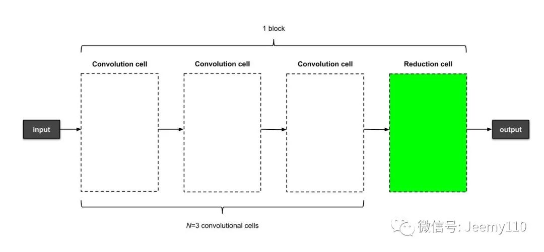
A sub-model contains multiple components. Each component contains N convolutional units and 1 down-sampling unit. Each convolution or down-sampling unit includes B nodes. Each node consists of standard convolution operations. N and B are two hyperparameters that can be adjusted.

Below is a sub-model with 3 components. Each component contains N=3 convolutional units and 1 down-sampling unit. The operations in each unit are not listed here.

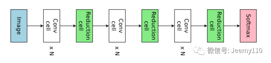
Overview of the generated final network.

1.2.2 Generating Sub-models from Micro Search

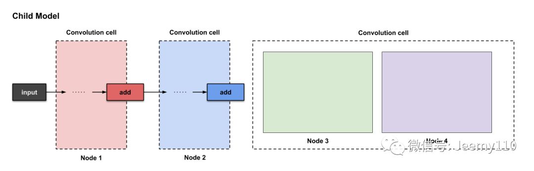
For simplicity, let’s first build a sub-model containing only a single component. Each component contains N=3 convolutional units and 1 down-sampling unit. Each unit contains B=4 nodes. Therefore, the generated sub-model should look like the following:

A sub-model generated from micro search, containing one component, with each component containing 3 convolutional units and one down-sampling unit. The operations in each unit are not listed here.

1.2.3 Fast Forward

Next, we will introduce how to construct the following two convolutional units. Note that each unit ultimately performs an add operation.

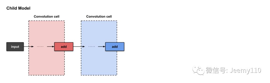
The two convolutional units constructed in micro search

1.2.4 Convolutional Unit #3

Now, let’s prepare the third convolutional unit together.

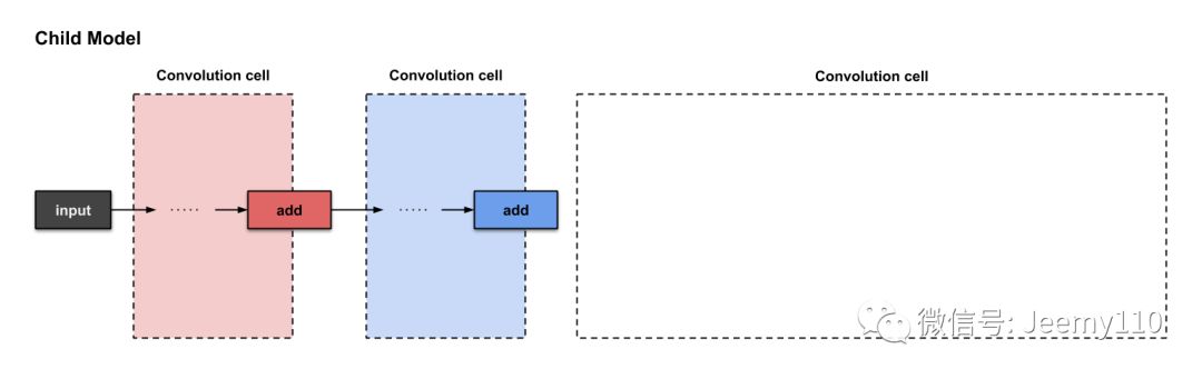
The preparation of the third convolutional unit in micro search

Each convolutional unit is assumed to have four nodes. The first two nodes are actually the current unit’s previous two units. The remaining two nodes are constructed from what we are about to build. Below are the labeled nodes.

The corresponding four nodes when constructing Convolutional Unit #3

From this point on, you can forget the label “convolutional unit” and focus only on the label “node.” If you want to know whether these nodes will change when constructing each convolutional unit, the answer is yes. Each unit will allocate nodes in this behavior.

You may also wonder, since we have already constructed operations in nodes 1 and 2 (i.e., units 1 and 2), what else needs to be constructed in these nodes? Good question!

1.2.5 Convolutional Unit #3: Node 1 (Red) and Node 2 (Blue)

For each unit we construct, the first two nodes do not necessarily need to be constructed, but they should serve as inputs for the other nodes. In our case, since we constructed four nodes, nodes 1 and 2 become the inputs for nodes 3 and 4. Therefore, we do not need to do anything for nodes 1 and 2; we just need to continue constructing nodes 3 and 4.

1.2.6 Convolutional Unit #3: Node 3 (Green)

We start constructing the unit from node 3. Unlike in macro search, where the controller needs to select two decisions, in micro search, the controller needs to select four decisions (or two pairs of decisions).

• Two nodes to connect

• Two operations for each of the two nodes to connect

Based on these four decisions, the controller will execute four times. Below is the execution process:

The outputs of the first four steps from the controller are (2, 1, avg5×5, sep5×5), used to construct node 3

From the above image, we can see that the controller selected 2, 1, avg5×5, sep5×5 from the first four execution outputs. How do these decisions translate into the structure of the sub-model? As follows:

How the controller’s first four outputs 2, 1, avg5×5, sep5×5 are translated into constructing node 3

From the above image, we can see that three things happen:

1. The output of node 2 (blue) performs the avg5×5 operation.

2. The output of node 1 (red) performs the sep5×5 operation.

3. The results of the above two operations execute an add operation together.

1.2.7 Convolutional Unit #3: Node 4 (Purple)

For node four, we repeat the same steps. Now the controller has three nodes (nodes 1, 2, and 3) to choose from. Below, the controller generates 3, 1, id, avg3×3.

The outputs of the controller’s first four steps are (3, 1, id, avg3×3), used to construct node 4

The translation and construction process is as follows:

How the controller’s first four outputs 3, 1, id, avg3×3 are translated into constructing node 4

From the above image, we can see that three things happen:

1. The output of node 3 (green) performs the id operation.

2. The output of node 1 (red) performs the avg3×3 operation.

3. The results of the above two operations execute an add operation together.

1.2.8 Down-sampling Unit

Remember that for every N convolutional units, we need one down-sampling unit? In this tutorial, N=3, and we just constructed the third convolutional unit, so it’s time to build a down-sampling unit. As mentioned earlier, the design of the down-sampling unit is very similar to that of the convolutional unit, with the only difference being that the stride of those operations is 2.

1.2.9 Conclusion

This is the entire process of generating sub-models using micro search. I hope the content is not too overwhelming for you (the readers); I felt this way when I first read this article.

Notes

Based on the joint probability distribution defined by probabilistic graphical models, we can infer the marginal distribution of the target variable or the conditional distribution given certain observable variables.

Since this article mainly discusses macro search and micro search, I (the author) have not mentioned many small details (especially regarding transfer learning). Briefly, here are some points:

• Where is ENAS efficient? Answer: Transfer learning. If the computational process between two nodes has already been completed (trained), the weights of the convolution kernel and 1×1 convolution (used to maintain the output channel count, which was not mentioned earlier) will be reused. This is why ENAS is faster than its predecessors.

• When skip connections are not needed, the controller can still select decisions.

• For the controller, there are six available operations: convolution with kernel sizes of 3×3 and 5×5, depthwise-separable convolution, max pooling with a kernel size of 3×3, and average pooling.

• Understand the concatenation operation at the end of each unit, which is used to tie up any loose ends of nodes.

• Briefly understand the policy gradient algorithm (REINFORCE) in reinforcement learning.

Conclusion

4.1 Macro Search (For the Entire Network)

The final sub-model is shown below: