Source: Artificial Intelligence AI Technology


This article is about 6000 words long and is recommended to read in 12 minutes.
This article introduces your understanding of CNN and RNN.
This article mainly focuses on understanding CNN and RNN, summarizing their advantages through comparison while deepening one’s understanding of this area of knowledge. The code references are taken from the VQA model for processing images and text.
1. Introduction to CNN
CNN is a type of neural network that utilizes convolutional calculations. It can reduce large images with many pixels to smaller pixel images while retaining the main features. This article elaborates on the content from Professor Li Hongyi’s PPT.
1.1 Why CNN for Images
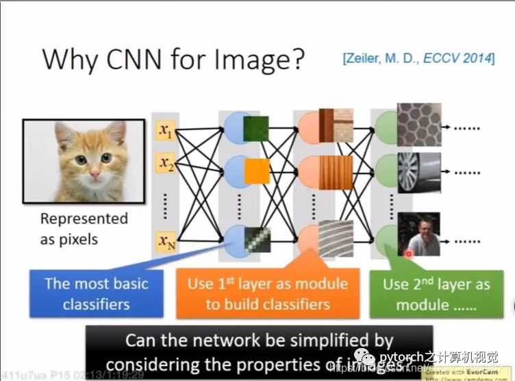
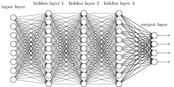
① Why Introduce CNN?Image illustration: Given an image input into a fully connected neural network, the first hidden layer identifies whether there is green present, whether there is yellow, or if there are diagonal stripes. The second hidden layer combines the outputs of the first hidden layer to achieve more complex functions. For example, if it sees a vertical line and a horizontal line, it recognizes part of a box; if it sees brown and stripes, it recognizes wood grain; if it sees diagonal stripes and green, it recognizes part of a gray stripe. Based on the output of the second hidden layer, if a neuron sees a honeycomb, it activates, and if it sees a person, it activates.However, if we generally use a fully connected neural network, we would need many parameters. For example, if the input vector is 30,000 dimensions and the first hidden layer has 1,000 neurons, then the first hidden layer would have 30,000*1,000 parameters, resulting in a very large amount of data, leading to low computational efficiency and accuracy. The introduction of CNN primarily solves these problems and simplifies our neural network architecture. Some weights may not be needed, and CNN uses filtering methods to filter out unnecessary parameters, retaining important parameters for image processing.② Why Use Fewer Parameters for Image Processing?Three characteristics:
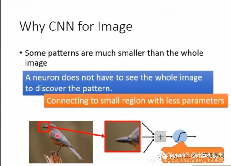
Most patterns are smaller than the entire image, so a neuron does not need to observe the entire image but only a small part of it to find a desired pattern. For example, given an image, a neuron in the first hidden layer looks for the beak of a bird, while another neuron looks for the bird’s claws. As shown in the image, it only needs to look at the red box and does not need to observe the entire image to find the bird’s beak.
Different positions of the bird’s beak only require training one parameter to recognize the beak; there is no need to train separately.
We can use subsampling to reduce the size of the image without changing the target image.
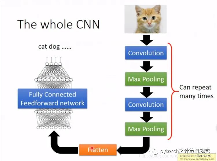
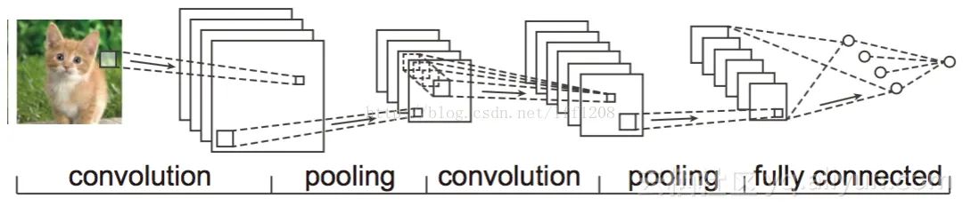
1.2 CNN Architecture Diagram
The first two properties in section 1.1 require convolution calculations, while the last pooling layer processes them, which will be introduced in detail in the next section.
1.3 Convolutional Layer
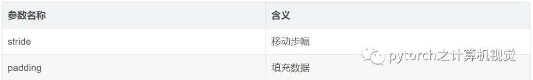
1.3.1 Important Parameters
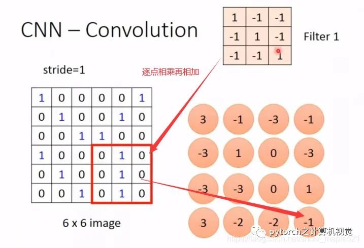
1.3.2 Convolution Calculation
The matrix convolution calculation is as follows:The calculation is as follows: the input image has a pixel value of 553, and after padding=1, it forms a pixel value of 773. The convolution kernel is of size 333, with 2 convolution kernels and a stride of 2. Note that the depth of the convolution kernel must match the depth of the incoming pixel values. When the blue position number scanned corresponds to the red position number of the convolution kernel, they are multiplied and summed to get the data at the green position.The change in pixel number is: (n+2p-f)/s = (5+2-3)/2 + 1= 3 resulting in 332 data. The output pixel depth after convolution equals the number of convolution kernels from the previous layer. This result is used as the input value for the pooling layer.Typically, the size of the convolution kernel is chosen to be odd. The depth must be the same as the depth of the pixel values output from the previous layer, such as a convolution kernel of size 3*3*3, while the output pixel depth equals the number of convolution kernels in this convolution. This point should not be confused.
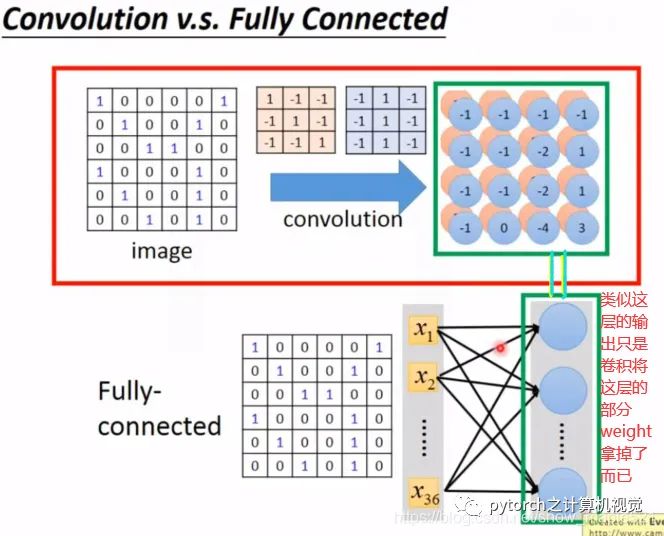
1.3.3 Relationship Between Convolutional Layer and Fully Connected Layer
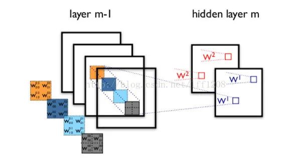
In fact, convolution is simply removing some weights from the fully connected layer. The output result calculated by the convolutional layer is actually the output of the hidden layer of the fully connected layer. As shown in the figure:Convolution does not consider all features of the input; it only relates to the features that pass through the filter. As shown below: a 6*6 image is unfolded into 36 pixels, and the next layer only relates to 9 pixels of the input layer, not all connections, thus using very few parameters. The specific diagram is as follows:From the above figure, it can also be seen that the calculations for 3 and -1 do not require different weights like a fully connected network; instead, the weights for these calculations are the same, which is known as parameter sharing.
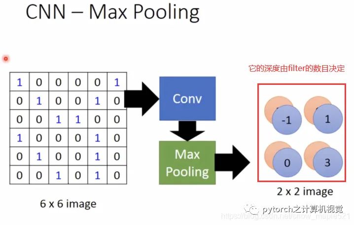
1.4 Pooling Layer
Based on the matrix from the previous convolution calculation, pooling is performed (merging four values within a box into one value, taking the maximum or average), as shown in the figure:After one convolution and one pooling, the original 6×6 image is transformed into a 2×2 image.
1.5 Applications
Mainly using the PyTorch framework to introduce convolutional neural networks.Source code:
torch.nn.Conv2d(in_channels: int, # Number of input image channels
out_channels: int, # Number of output channels generated by convolution
kernel_size: Union[T, Tuple[T, T]], # Size of the convolution kernel
stride: Union[T, Tuple[T, T]] = 1, # Stride of the convolution, default: 1
padding: Union[T, Tuple[T, T]] = 0, # 0 padding added to both sides of input, default: 0
dilation: Union[T, Tuple[T, T]] = 1, # Spacing between kernel elements, default: 1
groups: int = 1, # Number of blocked connections from input channels to output channels, default: 1
# groups: controls the connection between input and output; the number of input and output channels must be divisible by groups.
# When groups=1: all inputs pass to all outputs
# When groups=2: equivalent to two convolution layers, each seeing half of the input channels and producing half of the output channels, combining the two.
# When groups=in_channels: each channel has its own set of filters, with a size of out_channel/in_channel
bias: bool = True, # Adds a learnable bias to the output, default: true
padding_mode: str = 'zeros')
# Note: kernel_size, stride, padding, dilation parameter types can be int or tuple. When it is a tuple, the first int is the height dimension, and the second is the width dimension. When it is a single int, height and width values are the same.
# Square kernel and equal stride
m = nn.Conv2d(16, 33, 3, stride=2)
# Non-square kernel and unequal stride and padding
m = nn.Conv2d(16, 33, (3, 5), stride=(2, 1), padding=(4, 2))
# Non-square kernel and unequal stride and padding and dilation
m = nn.Conv2d(16, 33, (3, 5), stride=(2, 1), padding=(4, 2), dilation=(3, 1))
input = torch.randn(20, 16, 50, 100)
output = m(input)
Application: Here, VGG16 is used, and the PyTorch torchsummary library is introduced, which can print out the network model, for example:
import torchvision.models as models
import torch.nn as nn
import torch
from torchsummary import summary

device = torch.device('cuda' if torch.cuda.is_available() else 'cpu')
model = models.vgg16(pretrained=True).to(device)
print(model)
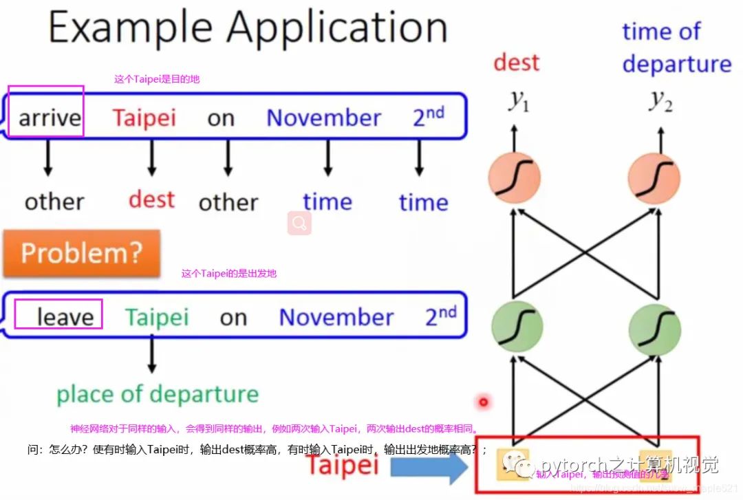
Every ticket booking system will have a slot filling; some slots are Destination, and some slots are time of arrival. The system needs to know which words belong to which slot; for example:
I would like to arrive Taipei on November 2nd; here, Taipei is the Destination, and November 2nd is the time of arrival;
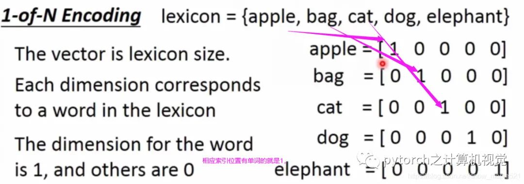
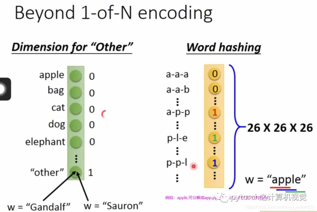
Using a regular neural network, we input the word Taipei into the network; of course, before inputting, we need to convert it into a vector representation. There are many ways to represent it; here we use: 1-of-N Encoding, represented as follows:Other word vector methods are as follows:However, if the following situation occurs, the system will make errors.Question: What should we do? Sometimes when inputting Taipei, the output probability for destination is high, and sometimes when inputting Taipei, the output probability for departure is high?Answer: At this point, our network needs to have “memory” to remember the previously input data. For example, when Taipei is the destination, it sees arrive; when Taipei is the departure, it sees leave. This type of memory network is called: Recurrent Neural Network (RNN)
2.2 Introduction to RNN
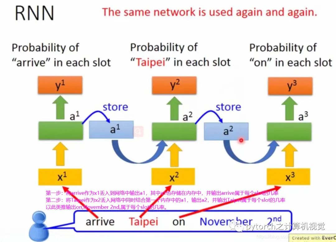
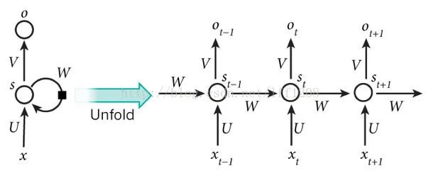
The hidden layer output of RNN will be stored in memory, and when the next input data comes in, it will use the last output stored in memory. The illustration is as follows:In the figure, the same weights are represented by the same color. Of course, the hidden layer can have many layers; the RNN introduced above is the simplest version, and the next section will introduce the enhanced version, LSTM.
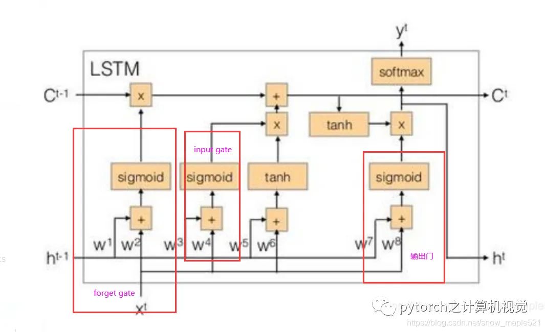
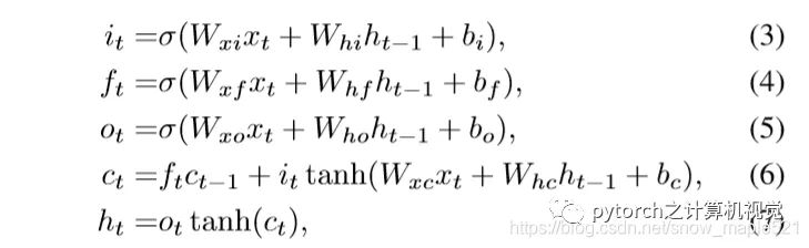
2.3 LSTM of RNN
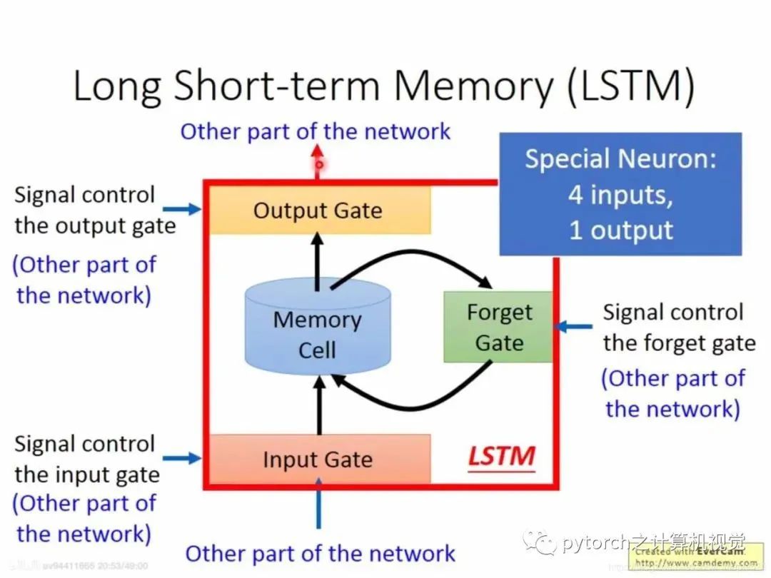
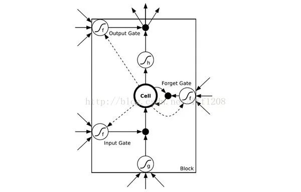
The commonly used memory is Long Short-Term Memory.When external information needs to be input into memory, a “gate”—input gate is required, and when the input gate opens and closes is learned by the neural network. Similarly, the output gate is also learned by the neural network, and the forget gate is the same.Thus, LSTM has four inputs and one output. The simplified diagram is as follows:The formulas are as follows:
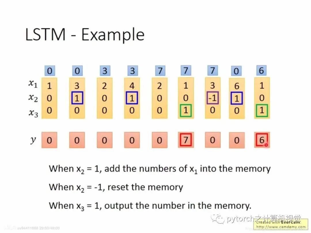
2.4 Example of LSTM
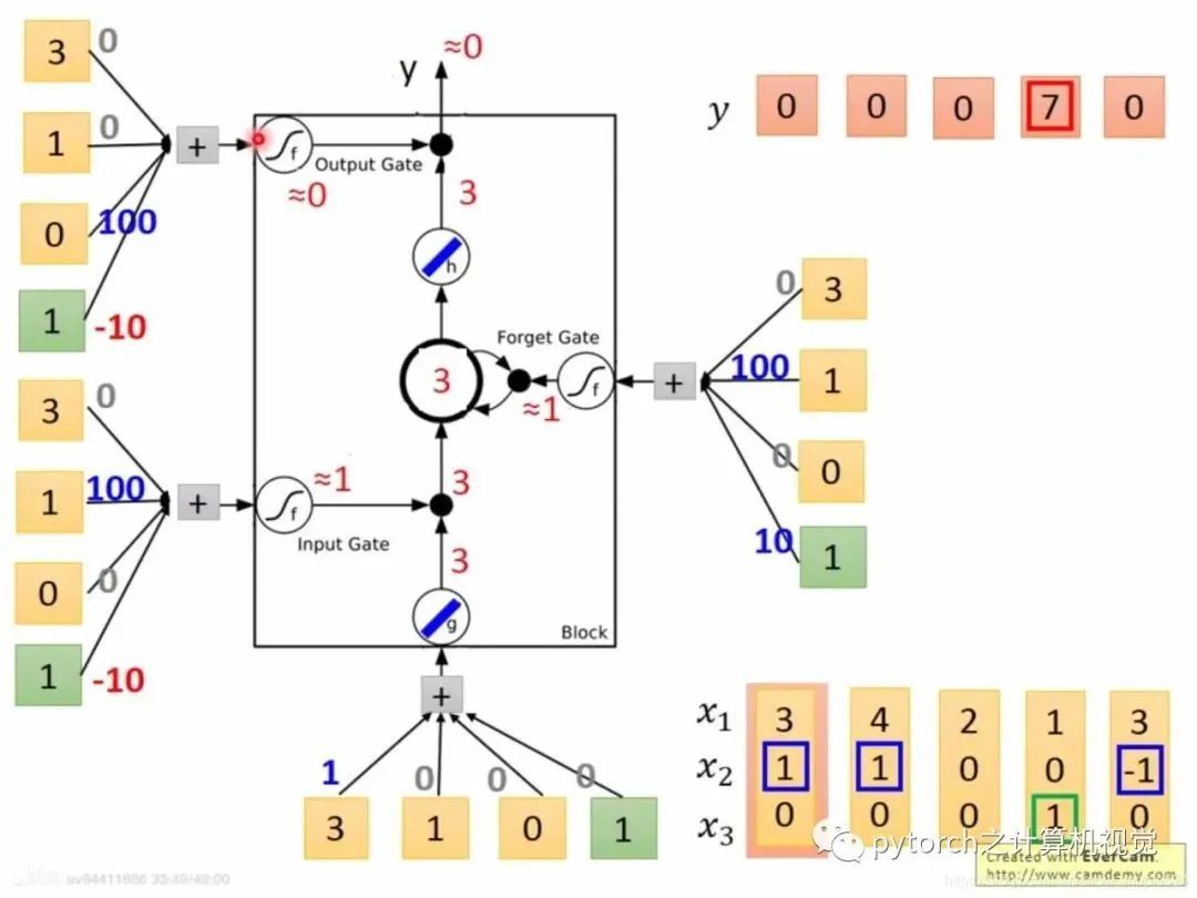
In the figure, x2 = 1 sends x1 into memory. If x2 = -1, it clears the values in memory. If x3 = 1, it outputs the data in memory. As shown in the figure, in the first column, x2 = 0 does not send to memory; in the second column, x2 = 1 sends the current x1 = 3 into memory (note that the data in memory is cumulative, for example, in the fourth column, x2 = 1, at this time x1 = 4, and the memory is 3, so together it is 7). In the fifth column, it is found that x3 = 1, so the output is the value in memory, which is 7.Combining the LSTM simplified diagram is as follows:Assuming the first column comes in: x1=3, x2=1, x3=0 steps: g—Tanh: x1w1+x2w2+x3w3 = 3 f—sigmoid: x1w1+x2w2+x3w3=90 sigmoid after=1. After calculating f and g, they are passed to input gate = 3*1=3, forget gate = 1, indicating no need to clear to 0, and x3 = 0, indicating the output gate is locked, so the output is still 0.
2.5 Practical Application of LSTM
The LSTM network is encapsulated in PyTorch, and you can directly use nn.LSTM, for example:
The differences between CNN and RNN are linked here, referencing a summary by the blog author, (https://blog.csdn.net/lff1208/article/details/77717149) as follows.
DNN Formation
To overcome gradient disappearance, activation functions like ReLU and maxout replaced sigmoid, forming the basic structure of DNN today. The structure is similar to a multi-layer perceptron, as shown in the figure:We see that in the structure of fully connected DNN, the lower layer neurons can connect with all upper layer neurons, leading to an explosion in the number of parameters. Assuming the input is a 1K*1K pixel image, and the hidden layer has 1M nodes, this layer alone has 10^12 weights to train, which not only easily leads to overfitting but also easily falls into local optima.
CNN Formation
Due to the inherent local patterns in images (such as eyes, noses, mouths in faces, etc.), the convolutional neural network CNN was introduced to combine image processing and neural networks. CNN links upper and lower layers via convolutional kernels, sharing the same convolutional kernel across all images, while preserving the original positional relationships through convolution operations.To simply illustrate the structure of convolutional neural networks, assume we need to recognize a colored image, which has four channels ARGB (opacity, red, green, blue, corresponding to four images of the same size). Assume the convolution kernel size is 100*100, and we use 100 convolution kernels w1 to w100 (intuitively, each convolution kernel should learn different structural features).Using w1 for convolution on the ARGB image generates the first image in the hidden layer; the first pixel in the upper left corner of this hidden layer image is the weighted sum of the pixels within the 100*/100 area of the four input images, and so on.Similarly, calculating with other convolution kernels results in 100 hidden layer images. Each hidden image corresponds to different features in the original image. Continuing this structure, CNN also includes max-pooling and other operations to further enhance robustness.Note that the last layer is actually a fully connected layer. In this example, we notice that the parameters from the input layer to the hidden layer have suddenly reduced to 100*100*100=10^6! This allows us to obtain a good model with the training data available. The suitability for image recognition, as mentioned by the user, is precisely due to the CNN model limiting the number of parameters and exploiting the characteristics of local structures. Following the same reasoning, utilizing local information in speech spectrogram structures, CNN can also be applied to speech recognition.
RNN Formation
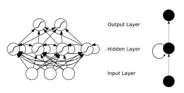
DNN cannot model changes over time series. However, the temporal order of samples is crucial for applications like natural language processing, speech recognition, and handwriting recognition. To meet this demand, another type of neural network structure has emerged—Recurrent Neural Network (RNN).In ordinary fully connected networks or CNNs, the signals of each layer of neurons can only propagate to the upper layer, and the processing of samples at various moments is independent, hence they are also called feed-forward neural networks. In RNN, the output of neurons can directly influence themselves in the next time period; that is, the input of the i-th layer neuron at time m includes not only the output of the (i-1)-th layer neuron at that time but also its own output at (m-1)! Represented in a diagram like this:For ease of analysis, it is unfolded over time segments as shown in the following diagram:
The final result O(t+1) of the network at time (t+1) is the result of the input at that moment and all historical influences! This achieves the goal of modeling time series. RNN can be seen as a neural network that transmits over time, where its depth is the length of time! As mentioned above, the “gradient disappearance” phenomenon will also occur, but this time it happens along the time axis.Therefore, RNN has a problem of not being able to solve long-term dependencies. To solve the above issues, LSTM (Long Short-Term Memory) was proposed, which implements memory functions over time through gate controls and prevents gradient disappearance. The structure of LSTM units is shown in the diagram below:In addition to DNN, CNN, RNN, ResNet (Deep Residual), and LSTM, there are many other structures of neural networks. For instance, in sequence signal analysis, if I can predict the future, it will also help with recognition.This has led to the development of bidirectional RNNs and bidirectional LSTMs, which utilize both historical and future information.In fact, regardless of the type of network, they are often used in combination in practical applications. For example, CNN and RNN often connect a fully connected layer before the upper layer output, making it difficult to determine which category a particular network belongs to. It is not hard to imagine that as the popularity of deep learning continues, more flexible combinations and more network structures will be developed.A simple summary is as follows:Editor: Yu TengkaiProofreader: Lin Yilin