
Click on the above“Beginner’s Guide to Vision” to choose to add Star or Pin.
Important content delivered promptly
Using mature frameworks like Tensorflow and PyTorch to implement Recurrent Neural Networks (RNNs) has greatly lowered the technical barriers to entry.
However, for beginners, this is still far from enough. Understanding the why is just as important as understanding the how.

To avoid basic mistakes, it is essential to build a solid theoretical foundation and then use RNNs to solve more practical problems.
So, here’s an interesting question to ponder:
How would you construct an RNN using only NumPy, without frameworks like TensorFlow?
Don’t worry if you’re at a loss. Here’s a tutorial: constructing an RNN for the NLP domain from scratch using NumPy.
This will guide you through the RNN construction process.
Initialize Parameters
Unlike traditional neural networks, RNNs have three weight parameters, namely:
Input weights, internal state weights, and output weights.
First, initialize the three parameters with random values.
Next, initialize the word embedding dimension and output dimension to 100 and 80, respectively.
The output dimension is the total number of unique word vectors present in the vocabulary.
hidden_dim = 100
output_dim = 80 # this is the total unique words in the vocabulary
input_weights = np.random.uniform(0, 1, (hidden_dim,hidden_dim))
internal_state_weights = np.random.uniform(0,1, (hidden_dim, hidden_dim))
output_weights = np.random.uniform(0,1, (output_dim,hidden_dim))
The variable prev_memory refers to the internal state (these are the memories from previous sequences).
Other parameters are also initialized with values.
The gradients for input_weight, internal_state_weight, and output_weight are named dU, dW, and dV, respectively.
The variable bptt_truncate indicates the number of timestamps the network must backtrack during backpropagation to overcome the vanishing gradient problem.
prev_memory =  np.zeros((hidden_dim,1))
learning_rate = 0.0001
nepoch = 25
T = 4   # length of sequence
bptt_truncate = 2
dU = np.zeros(input_weights.shape)
dV = np.zeros(output_weights.shape)
dW = np.zeros(internal_state_weights.shape)
Forward Propagation
Output and Input Vectors
For example, if the sentence is: I like to play., suppose in the vocabulary:
I is mapped to index 2, like corresponds to index 45, to corresponds to index 10, **corresponds to index 64, and punctuation.** corresponds to index 1.
To demonstrate the transition from input to output, we first randomly initialize the word embeddings for each word.
input_string = [2,45,10,65]
embeddings = [] # this is the sentence embedding list that contains the embeddings for each word
for i in range(0,T):
    x = np.random.randn(hidden_dim,1)
    embeddings.append(x)
The input is complete, and now we need to consider the output.
In this project, the RNN unit, after receiving the input, outputs the next most likely word.
To train the RNN, when the t+1th word is given as output, the tth word is used as input. For example, when the RNN unit outputs the word “like”, the input given is “I”.
Now the input is in the form of embedding vectors, while the output format required for calculating the loss function is a One-Hot vector.
This operation is performed for each word in the input string except the first word, as the neural network learns only from a sample sentence, with the initial input being the first word of that sentence.
The Black Box Computation of RNN
Now that we have the weight parameters and know the input and output, we can begin the forward propagation calculations.
Training the neural network requires the following calculations:
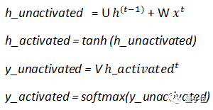
Where:
U represents input weights, W represents internal state weights, and V represents output weights.
The input weights are multiplied by input(x), and the internal state weights are multiplied by the previous layer’s activation (prev_memory).
The activation function used between layers is tanh.
def tanh_activation(Z):
     return (np.exp(Z)-np.exp(-Z))/(np.exp(Z)+np.exp(-Z)) # this is the tanh function can also be written as np.tanh(Z)
def softmax_activation(Z):
        e_x = np.exp(Z - np.max(Z))  # this is the code for softmax function
        return e_x / e_x.sum(axis=0)
def Rnn_forward(input_embedding, input_weights, internal_state_weights, prev_memory,output_weights):
    forward_params = []
    W_frd = np.dot(internal_state_weights,prev_memory)
    U_frd = np.dot(input_weights,input_embedding)
    sum_s = W_frd + U_frd
    ht_activated = tanh_activation(sum_s)
    yt_unactivated = np.asarray(np.dot(output_weights,  tanh_activation(sum_s)))
    yt_activated = softmax_activation(yt_unactivated)
    forward_params.append([W_frd,U_frd,sum_s,yt_unactivated])
    return ht_activated,yt_activated,forward_params
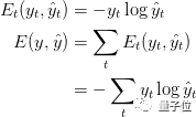
Calculating the Loss Function
Next, the loss function uses the cross-entropy loss function, given by the following formula:
def calculate_loss(output_mapper,predicted_output):
    total_loss = 0
    layer_loss = []
    for y,y_ in zip(output_mapper.values(),predicted_output): # this for loop calculation is for the first equation, where loss for each time-stamp is calculated
        loss = -sum(y[i]*np.log2(y_[i]) for i in range(len(y)))
        loss = loss/ float(len(y))
        layer_loss.append(loss)
    for i in range(len(layer_loss)): #this the total loss calculated for all the time-stamps considered together.
        total_loss  = total_loss + layer_loss[i]
    return total_loss/float(len(predicted_output))
The most important thing is that we need to see line 5 in the code above.
As is known, the ground_truth output (y) is in the form of [0, 0, …, 1, …0] and predicted_output (y^hat) is in the form of [0.34, 0.03, …, 0.45]. We need the loss to be a single value to infer the total loss.
To achieve this, the sum function is used to obtain the sum of the errors for each value in y and y^hat at a specific timestamp.
total_loss is the loss of the entire model (including all timestamps).
Backpropagation
The chain rule of backpropagation:
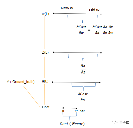
As shown in the figure above:
Cost represents the error, which indicates the difference between y^hat and y.
Since Cost is a function of the output, the change reflected by the activation a is represented by dCost/da.
In practice, this means looking at this change (error) value from the perspective of the activation node.
Similarly, the change of a with respect to z is represented as da/dz, and the change of z with respect to w is represented as dw/dz.
Ultimately, we care about how much the weights change (error).
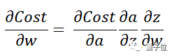
Since there is no direct relationship between the weights and Cost, the various relative change values in between can be multiplied directly (as shown in the above formula).
Backpropagation in RNN
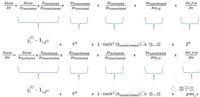
Since there are three weights in the RNN, we need three gradients. The gradients for input_weights (dLoss / dU), internal_state_weights (dLoss / dW), and output_weights (dLoss / dV).
The chain of these three gradients can be represented as follows:
The code for dLoss/dy_unactivated is as follows:
def delta_cross_entropy(predicted_output,original_t_output):
    li = []
    grad = predicted_output
    for i,l in enumerate(original_t_output): #check if the value in the index is 1 or not, if yes then take the same index value from the predicted_ouput list and subtract 1 from it.
        if l == 1:
    #grad = np.asarray(np.concatenate( grad, axis=0 ))
            grad[i] -= 1
    return grad
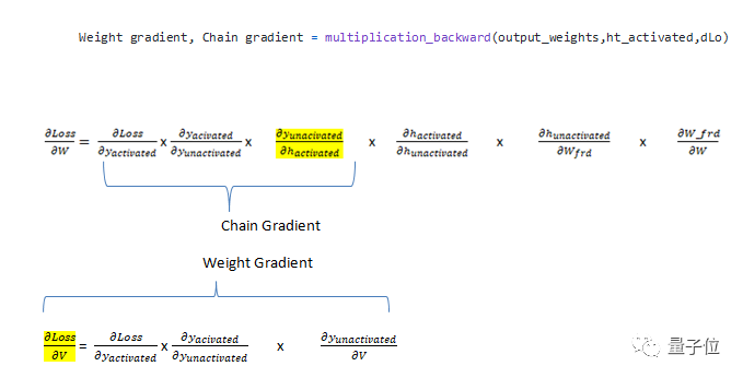
Calculate two gradient functions, one is multiplication_backward, and the other is addition_backward.
In the case of multiplication_backward, it returns two parameters: one is the gradient with respect to the weights (dLoss / dV), and the other is the chain gradient, which will become part of the chain for calculating the gradient of another weight.
In the case of addition_backward, when calculating the derivative, the derivatives of the components in the addition function (ht_unactivated) are all 1. For example: dh_unactivated / dU_frd=1 (h_unactivated = U_frd + W_frd), and the derivative of dU_frd / dU_frd is 1.
Therefore, only these two functions are needed to calculate the gradients. The multiplication_backward function is used for equations involving vector dot products, while addition_backward is used for equations involving the addition of two vectors.
def multiplication_backward(weights,x,dz):
    gradient_weight = np.array(np.dot(np.asmatrix(dz),np.transpose(np.asmatrix(x))))
    chain_gradient = np.dot(np.transpose(weights),dz)
    return gradient_weight,chain_gradient

def add_backward(x1,x2,dz):    # this function is for calculating the derivative of ht_unactivated function
    dx1 = dz * np.ones_like(x1)
    dx2 = dz * np.ones_like(x2)
    return dx1,dx2

def tanh_activation_backward(x,top_diff):
    output = np.tanh(x)
    return (1.0 - np.square(output)) * top_diff
At this point, we have analyzed and understood the backpropagation of RNN, which currently implements its function on a single timestamp. It can then be used to compute gradients across all timestamps.
As shown in the code below, forward_params_t is a list containing the forward parameters of the network for a specific time step.
The variable ds is a crucial part, as this line of code considers the hidden state from previous timestamps, which will help extract the information needed during backpropagation.
def single_backprop(X,input_weights,internal_state_weights,output_weights,ht_activated,dLo,forward_params_t,diff_s,prev_s):# include all the param values for all the data that's there
    W_frd = forward_params_t[0][0]
    U_frd = forward_params_t[0][1]
    ht_unactivated = forward_params_t[0][2]
    yt_unactivated = forward_params_t[0][3]
    dV,dsv = multiplication_backward(output_weights,ht_activated,dLo)
    ds = np.add(dsv,diff_s) # used for truncation of memory
    dadd = tanh_activation_backward(ht_unactivated, ds)
    dmulw,dmulu = add_backward(U_frd,W_frd,dadd)
    dW, dprev_s = multiplication_backward(internal_state_weights, prev_s ,dmulw)
    dU, dx = multiplication_backward(input_weights, X, dmulu) #input weights
    return (dprev_s, dU, dW, dV)
For RNNs, due to the vanishing gradient problem, truncated backpropagation is used instead of the original.
In this technique, the current unit will only look at k timestamps rather than just one timestamp, where k indicates the number of previous units to backtrack.
def rnn_backprop(embeddings,memory,output_t,dU,dV,dW,bptt_truncate,input_weights,output_weights,internal_state_weights):
    T = 4
    # we start the backprop from the first timestamp.
    for t in range(4):
        prev_s_t = np.zeros((hidden_dim,1)) #required as the first timestamp does not have a previous memory,
        diff_s = np.zeros((hidden_dim,1)) # this is used for the truncating purpose of restoring a previous information from the before level
        predictions = memory["yt" + str(t)]
        ht_activated = memory["ht" + str(t)]
        forward_params_t = memory["params"+ str(t)]
        dLo = delta_cross_entropy(predictions,output_t[t]) #the loss derivative for that particular timestamp
        dprev_s, dU_t, dW_t, dV_t = single_backprop(embeddings[t],input_weights,internal_state_weights,output_weights,ht_activated,dLo,forward_params_t,diff_s,prev_s_t)
        prev_s_t = ht_activated
        prev = t-1
        dLo = np.zeros((output_dim,1)) #here the loss derivative is turned to 0 as we do not require it for the truncated information.
        # the following code is for the truncated bptt and its for each time-stamp.
        for i in range(t-1,max(-1,t-bptt_truncate),-1):
            forward_params_t = memory["params" + str(i)]
            ht_activated = memory["ht" + str(i)]
            prev_s_i = np.zeros((hidden_dim,1)) if i == 0 else memory["ht" + str[prev]]
            dprev_s, dU_i, dW_i, dV_i = single_backprop(embeddings[t] ,input_weights,internal_state_weights,output_weights,ht_activated,dLo,forward_params_t,dprev_s,prev_s_i)
            dU_t += dU_i #adding the previous gradients on lookback to the current time sequence
            dW_t += dW_i
        dV += dV_t
        dU += dU_t
        dW += dW_t
    return (dU, dW, dV)
Weight Updates
Once the gradients are computed using backpropagation, updating the weights is imperative, and this is done through batch gradient descent.
def gd_step(learning_rate, dU,dW,dV, input_weights, internal_state_weights,output_weights ):
    input_weights -= learning_rate* dU
    internal_state_weights -= learning_rate * dW
    output_weights -=learning_rate * dV
    return input_weights,internal_state_weights,output_weights
Training Sequence
Having completed all the above steps, you can now start training the neural network.
The learning rate used for training is static, but dynamic methods for changing the learning rate, such as step decay, can also be used.
def train(T, embeddings,output_t,output_mapper,input_weights,internal_state_weights,output_weights,dU,dW,dV,prev_memory,learning_rate=0.001, nepoch=100, evaluate_loss_after=2):
    losses = []
    for epoch in range(nepoch):
        if(epoch % evaluate_loss_after == 0):
                output_string,memory = full_forward_prop(T, embeddings ,input_weights,internal_state_weights,prev_memory,output_weights)
                loss = calculate_loss(output_mapper, output_string)
                losses.append(loss)
                time = datetime.now().strftime('%Y-%m-%d %H:%M:%S')
                print("%s: Loss after  epoch=%d: %f" % (time,epoch, loss))
                sys.stdout.flush()
        dU,dW,dV = rnn_backprop(embeddings,memory,output_t,dU,dV,dW,bptt_truncate,input_weights,output_weights,internal_state_weights)
        input_weights,internal_state_weights,output_weights= sgd_step(learning_rate,dU,dW,dV,input_weights,internal_state_weights,output_weights)
    return losses

losses = train(T, embeddings,output_t,output_mapper,input_weights,internal_state_weights,output_weights,dU,dW,dV,prev_memory,learning_rate=0.0001, nepoch=10, evaluate_loss_after=2)
Congratulations! You have now implemented an RNN from scratch!
Now, it’s time to move on to advanced architectures like LSTM and GRU.
Good news!
The Beginner's Guide to Vision knowledge circle is now open to the public👇👇👇


Download 1: OpenCV-Contrib Extension Module Chinese Version Tutorial
Reply "Extension Module Chinese Tutorial" in the background of the "Beginner's Guide to Vision" public account to download the first OpenCV extension module tutorial in Chinese on the internet, covering installation of extension modules, SFM algorithms, stereo vision, object tracking, biological vision, super-resolution processing, and more than twenty chapters of content.

Download 2: Python Vision Practical Project 52 Lectures
Reply "Python Vision Practical Projects" in the background of the "Beginner's Guide to Vision" public account to download 31 practical vision projects including image segmentation, mask detection, lane line detection, vehicle counting, eye line addition, license plate recognition, character recognition, emotion detection, text content extraction, and face recognition, helping to quickly learn computer vision.

Download 3: OpenCV Practical Project 20 Lectures
Reply "OpenCV Practical Project 20 Lectures" in the background of the "Beginner's Guide to Vision" public account to download 20 practical projects based on OpenCV, achieving advanced learning of OpenCV.

Group Chat

Welcome to join the reader group of the public account to exchange with peers. Currently, there are WeChat groups for SLAM, 3D vision, sensors, autonomous driving, computational photography, detection, segmentation, recognition, medical imaging, GAN, algorithm competitions, etc. (will gradually be subdivided in the future). Please scan the WeChat account below to join the group, and note: "Nickname + School/Company + Research Direction", for example: "Zhang San + Shanghai Jiao Tong University + Vision SLAM". Please follow the format when noting, otherwise it will not be approved. After successfully adding, you will be invited to relevant WeChat groups based on research direction. Please do not send advertisements in the group, otherwise you will be removed from the group, thank you for your understanding~