From:Number Theory Legacy

The prerequisite knowledge for this article includes:Recurrent Neural NetworksRNN, Word EmbeddingsWordEmbedding, Gated UnitsVanillaRNN/GRU/LSTM.

1 Seq2Seq

Seq2Seq is the abbreviation for sequence to sequence. The first sequence is called the encoder encoder, which is used to receive the source sequence source sequence. The second sequence is called the decoder decoder, which is used to output the predicted target sequence target sequence.

Seq2Seq is mainly used for sequence generation tasks, such as: machine translation, text summarization, dialogue systems, etc. Of course, it can also be used for tasks like text classification.

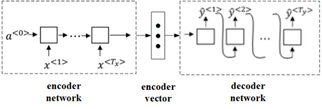
Figure 1.1 Seq2Seq

The most traditional Seq2Seq process is shown in Figure 1.1:

(1) Input the source sequence into the encoder network.

(2) The encoder encodes the information of the source sequence into a fixed-length vector encoder vector.

(3) The encoder vector is sent to the decoder network.

(4) The decoder outputs the predicted target sequence based on the input vector information.

After being proposed, Seq2Seq immediately received widespread attention and application, but also exposed some problems. The first to be noticed was that it was difficult to perfectly decode the entire text sequence compressed into a single vector by the encoder without any information loss.

Moreover, due to the characteristics of Recurrent Neural Networks RNN, the later the text is input in the source sequence, the greater its influence on the encoder vector. In other words, the encoder vector will contain more information from the tail of the sequence while neglecting the information from the head of the sequence. Therefore, in many early papers, the text sequence would be reversed before inputting into the encoder, and the model’s evaluation score would significantly improve.

To allow the decoder to better extract information from the source sequence, Bahdanau proposed the attention mechanism Attention Mechanism in 2014, and Luong improved the Bahdanau Attention in 2015. These are the two most classic attention mechanism models. The essence of the two Attention models is the same, and the following text will take the Luong Attention model as an example.

2 Attention Mechanism

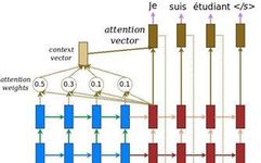
Understanding the attention mechanism can refer to the ideas in the CV field: when we see a painting, there is always a focus at every moment, such as a person, an object, or an action.

Therefore, in the NLP field, when we use the decoder to predict the output target sequence, we also hope to have a mechanism that associates the current step of the target sequence with certain steps of the source sequence.

For example, in the translation task, translating “我爱机器学习” into “I love machine learning.” at the first step of the decoder output sequence, we hope to focus on the input sequence’s “我” and translate “我” to “I“; at the third step, we hope to focus on “机器” and translate it to “machine“.

This example is relatively simple, and we might have a preliminary idea: could we translate each word in the source sequence into English individually and output them in order to form the target sequence?

However, if we think further, we will find two problems:

(1) Polysemy: The same word in the source sequence may have different outputs in the output sequence depending on the context. For example, “我” may be translated as “I” or “me“. This is somewhat similar to the Chinese “一词多义”, which in English might be called “one word, multiple forms”. We can broadly refer to this phenomenon, where one word can map to multiple words, as “polysemy”. An effective way to solve the polysemy problem is to refer to the contextual information of the source sequence, i.e., the context information, to generate word embeddings.

(2) Sequence Order: The source sequence and target sequence are not necessarily mapped in order, for example, “你是谁？” translates to “who are you?“. Different languages have different grammatical rules and orders. This requires determining which word in the source sequence should be translated at each step of the decoder output.

These two issues are the focus of the Attention mechanism.

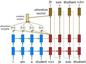
Figure 2.1 Luong Attention

Figure 2.1 is a diagram of Luong Attention, presented in a subsequent paper by the author.

Another way to understand Attention is to refer to the residual network ResNet. Because the source sequence is too long, early information cannot be effectively transmitted, so an additional channel is needed to send early information to the decoder. When sending, it should not only send one word’s information but also provide the contextual information.

The next section will introduce the implementation steps of the Attention mechanism using the simplest model. Before that, let’s agree on the parameter symbols:

h(output): RNN’s hidden state, mainly used to output information to RNN model.

s(state): RNN’s state, mainly used within the RNN model to pass information to the next step.

a: alignment vector

c: context information vector.

x: source sequence.

y: target sequence.

The subscripts indicates the source sequence, and the subscriptt indicates the target sequence. s1 indicates the first step in the source sequence, and so on.

The output and state in parentheses are for the reader to connect the algorithm theory in the paper with the industrial practice of tensorflow’s tf.nn.dynamic_rnn function. Just having a slight impression is sufficient. The dynamic_rnn function returns two vectors, the first being output, which is the h output of all steps of the encoder, and the second being state, which is the s output of the last step of the encoder.

3 Attention Quintessence

3.1 Execute Encoder

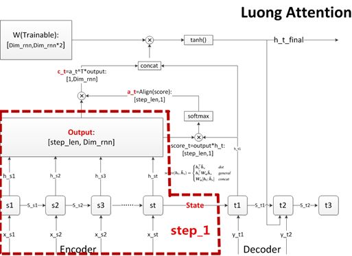
Figure 3.1 Step One: Execute Encoder

The action of step one is to sequentially input the source data into the Encoder and execute the Encoder. The purpose is to compile the information of the source sequence into a semantic vector for subsequent decoder use.

At each step, the encoder will output an output (h) vector representing the semantics of the current step and a state (s) vector:

(1) We collect the output (h) of each step to form the output matrix, which has dimensions of [step_len,dim_rnn], i.e. the length of the source data step multiplied by the number of rnn units.

(2) We collect the last step’s state (s) as the vector passed to the decoder.

The encoder contributes to the model by providing the outputs matrix and the state vector.

Note 1: For easier understanding, I used a single-layer network for the encoder, and the outputs and state of multi-layer networks can be seen in the description at the end of the previous section.

Note 2: Many papers do not have a unified standard for describing h and s, which often leads to confusion. Because the early papers’ RNN units were implemented using VanillaRNN or GRU, the h and s output at the same step are the same. However, if implemented using LSTM, h and s are different, which needs to be noted.

Note 3: In early papers, the encoder’s state was directly passed to the decoder as the initial state. However, in engineering applications, there are also cases where a 0 sequence is directly passed as the initial state to the decoder. Additionally, some papers also process the state by adding some extra information before passing it to the decoder. In summary, the way the state is passed between the encoder and decoder is quite flexible and can be chosen and improved according to actual situations.

Note 4: The number of units in the RNN is the dimension of the encoder output vector. It means using a dim_rnn dimensional vector to represent the semantic information of the text at the current step of the source sequence. Comparing this with the dimension dim_word_embd of the word vector that also represents semantic information, I suggest that the dimensions of the two should not differ too much; otherwise, it may lead to waste.

3.2 Calculate Alignment Coefficient a

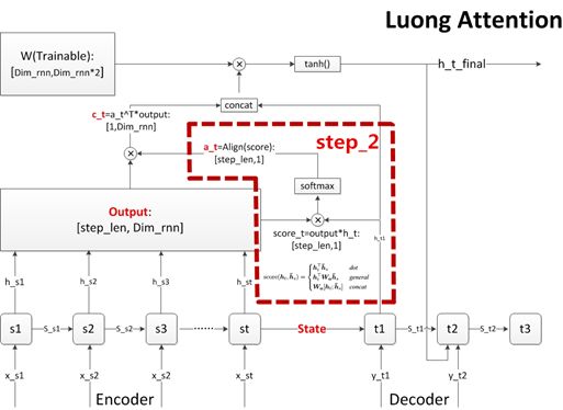
Figure 3.2 Step Two: Calculate Alignment Coefficient a

Step two addresses the “sequence order” problem proposed in section two. At each step of the decoder, we need to consider the relevance size between all steps of the source sequence and the current step of the target sequence, and output the corresponding (alignment) coefficient a.

Therefore, before the decoder outputs a prediction value, it will calculate a score for all steps of the encoder. This score indicates which steps of the encoder the current decoder needs to extract information from, as well as the weight of that extraction. Then, the score is summarized into a vector, allowing each decoder step to obtain a score vector with dimensions of [step_len,1].

There are many ways to calculate this score, and Figure 3.2 lists three traditional calculation methods mentioned in Luong Attention. The flowchart I drew uses the first method, which is to multiply the output (h) of all steps of the source sequence with the output (h) of the current step of the target sequence to obtain the score. Some papers innovate in the calculation method of the score.

After calculating the score, it is customary to use softmax for normalization to obtain the alignment vector a, which also has dimensions of [step_len,1].

Note 1: Many papers have different abbreviations for various parameters. A small trick to clarify the order of model processes is to look for the softmax function, using softmax as an anchor point. The common uses of softmax in Attention occur in two places: one is the alignment coefficient a in step two, and the other will be mentioned in step five, where the probability scores need to be normalized using softmax.

Note 2: Although the alignment coefficient a is merely a process data, it contains important information that can be used in PointerNet and CopyNet.

3.3 Calculate Context Semantic Vector c

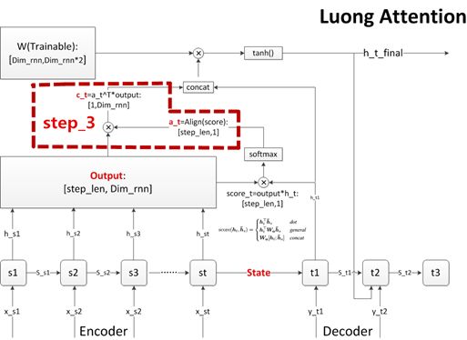
Figure 3.3 Step Three: Calculate Context Semantic Vector c

Before describing this step, let’s review the CBOW model of word vectors. After the CBOW model converges, the word vector of each word equals the average of the word vectors of several surrounding words. This implies that: what represents a word is not the word itself, but the context (environment) of the word.

The CBOW model is a rather straightforward way of averaging the context’s word vectors. In practice, if we can obtain the word vector in a weighted average manner, then this word vector can more accurately express the semantics of the word in the current context.

For example: “孔夫子经历了好几个春秋寒暑，终于修订完成了春秋麟史。” Here, the first “春秋” means “a year”; “经历” and “寒暑” are clearly more closely related to it, so when constructing the word vector using weighted context, it should be given a higher weight. The second “春秋” refers to one of the six classics of Confucianism, and “修订” and “麟史” are more closely related to it, so it should also be given a high weight.

In step three, we will use the alignment coefficienta as weights to perform a weighted sum of the output vectors of each step of the encoder (the alignment vectora dot-multiplied with the outputs matrix), resulting in the context semantic vector c for the current step of the decoder.

Note 1: BERT also employs the concept of alignment coefficients, and it is more intuitive and elegant.

3.4 Update Decoder State

Figure 3.4 Step Four: Update Decoder State

In step four, we need to update the decoder state, which can be h or s. The information data used to update h and s can include: the previous step’s s, the current step’s h, the current step’s context vector c, and other data containing effective information.

Bahdanau Attention and Luong Attention differ mainly in this step; the former updates s, while the latter updates h. However, since Bahdanau uses the previous step’s s and Luong uses the current step’s h, the latter is simpler to implement in engineering.

The specific details of the update formulas will not be described here, as different models may use different update formulas, and many papers innovate around the update formulas.

It is important to note that in this process, the training mode and prediction mode differ slightly: the decoder must input data at each step; in training mode, the input data is the true value of the target sequence at the current step, without using the previous step’s h; in prediction mode, the input data is the previous step’s h, without using the true value of the output sequence. Although I drew two inputs in Figure 3.4, one must be chosen based on whether the model is in training mode or prediction mode.

3.5 Calculate Output Prediction Word

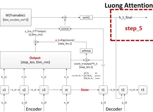
Figure 3.5 Step Five: Calculate Output Prediction Word

This step is not fully illustrated in the figure; it is actually quite simple. It is similar to the mapping from the semantic vector to the target word table in the CBOW model/Skip-Gram model, followed by performing softmax.

4 Others

4.1 Local Attention and Global Attention

The Attention mentioned earlier is all Global Attention, and there is also Local Attention, which will be briefly explained in this section.

Global Attention calculates the alignment coefficients a for all steps of the source sequence, while Local Attention only calculates the alignment coefficients a for part of the steps of the source sequence. The length of this part of steps is a hyperparameter that needs to be configured based on experience.

The selection (alignment) method for the center point of the part of steps captured by Local Attention is another point to focus on. The papers mention two alignment methods:

(1) Monotonicalignment (local-m): A simple and straightforward method that directly aligns the absolute values of the steps in the source and target sequences.

(2) Predictivealignment (local-p): This learns to calculate the alignment center of the truncated steps through the model.

Luong’s paper mentions that Local Attention performs better than Global Attention.

Note: In the CV field, there are Soft-Attention and Hard-Attention, which have similar advantages to the two Attention in the NLP field.

4.2 Commonly Replaceable Improvement Modules

1.Calculation methods for the scores score used to generate the alignment vector a.

2.Update formulas for h and s.

3.Basic RNN structures, including replacing gated units, changing RNN layers, and changing from unidirectional to bidirectional.

References

[1] Bahdanau D ,Cho K , Bengio Y . Neural Machine Translation by Jointly Learning to Align and Translate[J]. Computer Science, 2014.

[2] Luong M T ,Pham H , Manning C D . Effective Approaches to Attention-based Neural Machine Translation[J]. Computer Science, 2015.

[3] Andrew Ng Recurrent Neural Networks

Due to the word limit for WeChat articles, here is the link to the Zhihu article:https://zhuanlan.zhihu.com/p/73589030

Further updates or corrections will be presented in the Zhihu article.

Recommended Reading:

Attached is a PDF download of notes, detailed notes on MIT’s Chinese Linear Algebra course [Lesson Four]

Geometric Interpretation of Systems of Equations [MIT Linear Algebra Lesson One PDF Download]

PaddlePaddle Practical NLP Classic Model BiGRU + CRF Detailed Explanation