Recurrent Neural Networks (RNNs) based on long-range dependency modeling are widely used in various speech tasks, such as Keyword Spotting (KWS) and Speech Enhancement (SE). However, due to the power and memory limitations of low-resource devices, efficient RNN models are needed for practical applications.

In this paper, the author proposes an efficient RNN architecture called GhostRNN, which reduces hidden state redundancy through cheap operations.

Specifically, the author observes that certain parts of the hidden states in a trained RNN model are similar to others, indicating redundancy in specific RNNs.

To reduce redundancy and lower computational costs, the author proposes to first generate several intrinsic states and then apply cheap operations based on these intrinsic states to produce ghost states.

Experiments on KWS and SE tasks show that the proposed GhostRNN significantly reduces memory usage (by about 40%) and computational costs while maintaining similar performance.

1 Introduction

In recent years, with the rapid development of neural networks, significant improvements have been made in various speech tasks. Among these neural networks, RNNs, such as LSTMs [1] or GRUs [2], are widely used in various speech-related tasks on low-resource devices (e.g., mobile phones), such as KWS [3, 4, 5], SE [6], automatic speech recognition [7], acoustic echo cancellation [8, 9], etc., despite their lower parallelism compared to Transformers [10].

Due to the high demand for deploying AI models on edge devices with limited power and memory, it is desirable to design efficient models that maintain high performance while having low computational costs. Various efforts have been made in this direction. Dey and Salem [11] proposed an efficient variant of GRU that reduces the size of the gate matrix by adjusting the computation method of the gate matrix, for example, by calculating the gate vector using only the hidden state as input. The Light-Gated-GRU (Li-GRU) proposed in [12] removes the reset gate and evolves into a single-gate RNN. Amoh and Odame [13] proposed an embedded Gaed Recurrent Unit that has only one gate with a single-gate mechanism. Similar to Li-GRU, Fanta et al. [14] eliminated the reset gate in their proposed SITGRU and replaced the Tanh activation function with Sigmoid. Zhang et al. [15] used a dual-gate mechanism to compress RNN models. Although these methods effectively reduce the number of parameters in the model, reducing the number of gate matrices may impair the exploration of contextual information.

In this work, the author empirically observes the redundancy in the hidden states of RNN models, aside from the gate matrices in the previous studies mentioned above. Therefore, the author proposes to fully exploit the redundancy of hidden states to compress RNNs, which has not been researched in speech tasks. Specifically, the author considers RNN models in SE tasks and analyzes the hidden states in RNN layers.

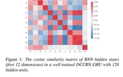
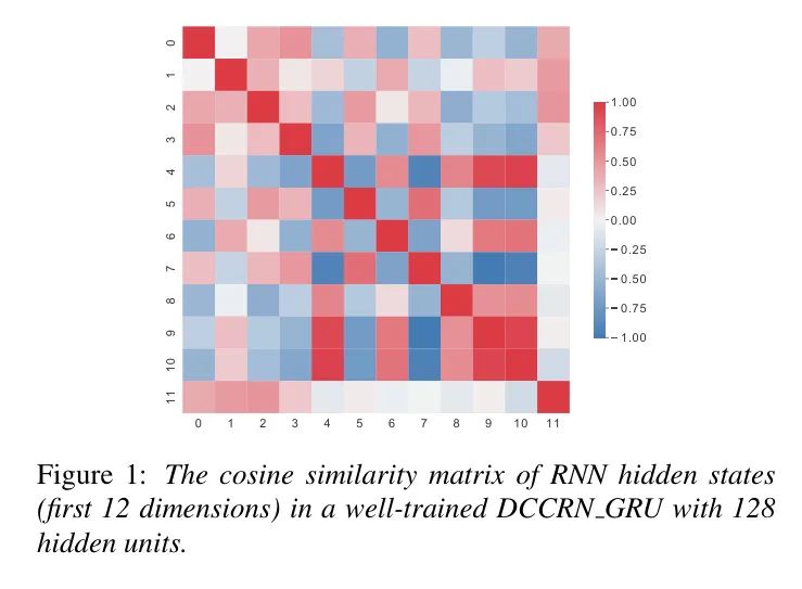
After n time steps, the feature map of the hidden state with m hidden units can be represented as the feature map of the i-th hidden unit. First, the author performs singular value decomposition on the hidden state feature map of a well-trained DCCRN_GRU model. The author finds that only half of the singular values can achieve a 99% contribution rate in Principal Component Analysis (PCA), indicating some relative redundancy. Additionally, as shown in Figure 1, the author computes the cosine similarity at different indices, where some similarity values are quite large, indicating high similarity [16].

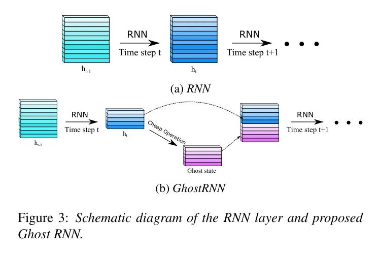
Inspired by the above observations, the author proposes GhostRNN to reduce redundancy in hidden states, thus constructing efficient RNN models. Specifically, part of the RNN hidden states is generated by a basic RNN model as intrinsic states. Next, several cheap operations, including simple linear transformations and activation functions, are implemented to generate ghost states based on the intrinsic states. Then, the ghost states are concatenated with the intrinsic states as the complete feature representation from the previous time step and passed to the next time step for further computation. Compared to the basic RNN matrix multiplication, the author’s cheap operations have fewer FLOPs and parameters, thus significantly reducing the computational and memory costs of the GhostRNN model.

Experiments were conducted on KWS and SE tasks to verify the effectiveness of the proposed method. The experimental results show that the author’s method achieves a 0.1% accuracy improvement on the Google Speech Command dataset while compressing the parameters of the Baseline model by 40%. In the SE task, the author’s method improves SDR and Si-SDR by about 0.1 dB at approximately 40% compression rate.

2 Proposed Method

This section details the proposed GhostRNN and illustrates model compression. For convenience, the author uses GRU to illustrate the definition of GhostRNN. The author’s method can be applied to other RNNs, such as LSTM.

RNN

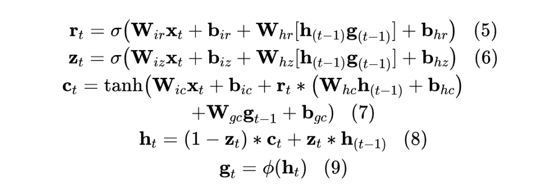
As a class of model structures, Recurrent Neural Networks (RNNs) utilize hidden states to store and utilize contextual information [17], including well-known variants such as Gated Recurrent Units (GRUs) and Long Short-Term Memory units (LSTMs). As one of the most commonly used RNN models, GRU is a simplified version of LSTM, defined as follows:

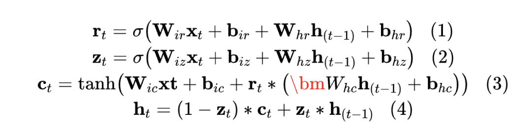
The reset gate, update gate, and candidate vector are represented as , and . and represent the hidden states at time step and time step, and are the input features at time step. As shown in Figures 1 to 4, the computation involves six matrices, where and have the same size, and and also have the same size. Additionally, the sizes of all matrices in the GRU model are closely related to the dimensions of the hidden states and input features. Therefore, an effective method to compress the parameters of the GRU model is to reduce the dimensionality of the hidden states. As mentioned in Section 1, by reducing the number of required gate vectors, the number of gate matrices can be reduced, leading to a decrease in the number of model parameters.

GhostRNN

To reduce hidden state redundancy, the proposed GhostRNN generates ghost states from intrinsic states using extremely low-cost transformations.

Observations on Hidden State Redundancy: As mentioned in the first part, previous research mainly focused on reducing the number of gate matrices when compressing models, with little attention paid to the redundancy of hidden states, which is also crucial for effectively reducing the number of model parameters. Therefore, this section will conduct a comprehensive study on the redundancy of hidden states. First, PCA contribution rate is used as an evaluation metric. The accumulated hidden state vectors over time are treated as feature maps and subjected to singular value decomposition. According to the results, only about half of the singular values are needed for the feature maps to achieve a 99% PCA contribution rate, indicating that complete feature information can be constructed using only half of the hidden states. Additionally, as shown in Figure 1, the author accumulates hidden state vectors of different dimensions at different time steps as state components and calculates the cosine similarity between different components. The results show that some components have cosine similarities close to 1. Figure 1(a) shows a set of components with highly correlated trends, indicating redundancy in the hidden states of GRU. On the other hand, as shown in Figure 1(b), the cosine similarity between specific components is close to 0, indicating that these state components are nearly orthogonal and thus necessary and irreplaceable. Therefore, retaining necessary state components and eliminating redundant components is a direct and practical way to compress RNN models.

Based on the above results and analysis, the author proposes the GhostRNN module, which constructs ghost states based on intrinsic states, as shown in Figure 3, and can be defined as follows:

Analysis on the Number of Parameters and Computational Complexity

The number of parameters in the ordinary GRU and the proposed GhostRNN can be calculated as follows:

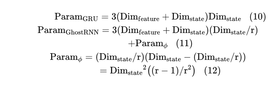
where represents the ratio of complete state to intrinsic state. As Eqs (10) to (11) show, the output hidden state dimension of GhostRNN is scaled by the ratio compared to that in the conventional GRU. Although an additional cheap operation module composed of linear layers is applied, according to Eq. (12), the number of parameters in the cheap operation module is much smaller than that in the GRU model. Therefore, the total number of parameters in GhostRNN will be compressed by a factor of .

If the cheap operation module is constructed using other computational methods (such as conventional linear transformations without parameters), the compression ratio can reach . Regarding computational complexity, since all matrices in GRU are linear layers, the computational complexity of GRU is almost proportional to the number of parameters. Therefore, the computational complexity of GhostRNN will also be reduced by the same factor .

3 Experiments

Two experiments were conducted to evaluate the effectiveness of the author’s method: KWS and SE.

Datasets

In the author’s experiments, the Google Speech Command dataset v0.02 [18] was used, which contains thousands of 1-second audio samples divided into 30 categories. Following previous research [3, 19], the author selected 12 categories: “yes,” “no,” “up,” “down,” “left,” “right,” “on,” “off,” “stop,” “go,” “mute,” and “unknown.” The author used 36,923, 4,445, and 4,890 samples of these for training, validation, and testing, respectively. The author used 10-dimensional Mel-frequency cepstral coefficients (MFCC) as speech features, with a window length of 40 ms and a window shift of 20 ms, resulting in a feature map size of 49×10 for each speech sample. Additionally, the author employed data augmentation techniques such as adding background noise and random shifts, as recommended in [3], to enhance model robustness.

To assess the performance of the author’s method in the SE task, the LibriMix dataset [20] was used, which generates noisy speech segments by combining clean speech from LibriSpeech [21] with noise from the WHA! dataset [22]. The author used the 16kHz version of the training-360 dataset, which consists of 50,800 training samples, 3,000 validation samples, and 3,000 test samples, totaling 234 hours of data. The author implemented the same data preprocessing as in Asteroid [23].

Settings and Evaluation Metrics

During the training process for KWS, the author used standard cross-entropy loss and the Adam optimizer with a batch size of 100. The author adopted a stepwise decreasing learning rate strategy, with an initial learning rate of 5e-4 and step sizes set at [10,000, 20,000]. All models were trained from scratch for a total of 30,000 iterations and evaluated using accuracy metrics [3]. To ensure the reliability of the author’s results, each model was trained three times with the same configuration, and the average experimental results were reported.

During the training process for SE, the author used permutation-invariant loss and the ADAM optimizer, setting the batch sizes to 12 (for DCRNN [5]) and 32 (for GRU-TasNet [24]). Learning rate decay strategies and early stopping strategies were applied in all experiments. The initial learning rate was set to 0.001 with a weight decay of 1e-5. In terms of filters, the author’s settings were consistent with those described in [23]. During evaluation, the author used five metrics: Signal-to-Noise Ratio (SDR), SDR improvement (SDRi), Scale-Invariant Signal-to-Noise Ratio (Si-SDR), Si-SDR improvement (Si-SDRi), and Short-Time Objective Intelligibility (STOI) [26].

Baselines

KWS model

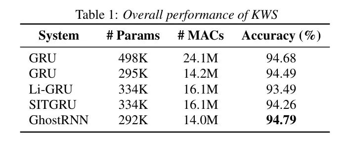
Table 1 shows that, as a baseline model for KWS [3], a GRU model of approximately 500k in size was used, along with another GRU model of approximately 295k in size, while also implementing Li-GRU [12] and SITGRU [14] for comparison.

SE models

To compare the SE task, the author selected two models as baseline models. The first is DCCRN [5], which primarily consists of convolutional layers supplemented by RNN layers. In the author’s experiments, the DCCRN-CL [5] model was chosen, and LSTM was replaced with GRU, selecting 128 and 80 hidden units to construct different sizes of baseline models.

GRU-TasNet. This model is optimized from the Time-domain Audio Separation Network, which consists of three parts: a 1-D convolutional encoder, a 1-D deconvolutional decoder, and a deep LSTM separation module [24]. In the author’s experiments, LSTM was replaced with GRU. The author designed four baseline models of different sizes, with differences based on the hidden layer sizes of GRU: 512, 384, 192, and 136.

Results on KWS

Table 1 presents the experimental results and model parameters. The proposed GhostRNN model was compared with two baselines: the 500k GRU and the 300k GRU, along with two other model compression methods: Li-GRU [12] and SITGRU [14]. The results indicate that the proposed GhostRNN model reduces parameters by approximately 40% while achieving about a 0.1% accuracy improvement compared to the 500k GRU model, also outperforming the slightly larger Li-GRU and SIT-GRU models, demonstrating the effectiveness of the proposed GhostRNN.

Results on SE

Table 2 shows the performance of DCCRN and DCCRN_Ghost128 on the libririx1 dataset. The results indicate that by pruning the hidden layer size in the GRU layer of the DCCRN model for model compression, the SDR and Si-SDR metrics decreased by about 0.1 dB. In contrast, when the author applied the proposed GhostRNN compression method and compressed approximately 10% of the parameters, the SDR and Si-SDR metrics decreased by only about 0.05 dB. These findings clearly demonstrate the effectiveness of GhostRNN.

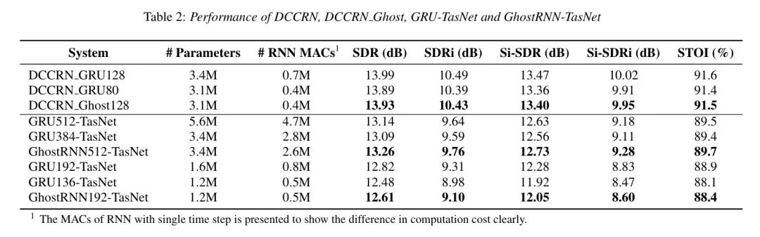
Table 2 presents the performance of GRU-TasNet and GhostRNN-TasNet on the libririx1 dataset. The metrics indicate that when the model is compressed from GRU512-TasNet to GRU384-TasNet, the SDR and Si-SDR slightly decrease, indicating redundancy in the parameters of GRU512-TasNet. In this case, the GhostRNN method achieves over 0.1 dB performance improvement in SDR and Si-SDR while reducing parameters by 40% compared to GRU512-TasNet. However, when the model is further compressed to 1.6M (GRU192-TasNet), performance significantly declines, indicating lower model redundancy. In this case, GhostRNN192 has about a 0.13 dB advantage over GRU136-TasNet in SDR and Si-SDR. Overall, GhostRNN is an effective RNN model compression method.

4 Conclusions

In this paper, the author proposed GhostRNN to compress RNN models based on the observed redundancy in hidden states. In the author’s GhostRNN, given the intrinsic hidden states, extremely low-cost Transformer Layers are applied to generate ghost states, significantly reducing the number of parameters and computational costs of the base GRU model while achieving competitive performance. Experimental results show that the author’s method achieves a 0.1% accuracy improvement on the Google Speech Command dataset while compressing the parameters of the baseline model. In the SE task, the author’s method improves SDR and Si-SDR by about 0.1 dB at a compression rate of about 40%.

Furthermore, the author’s method improves SDR and other evaluation metrics by approximately 0.13 dB compared to baseline GRU models with the same number of parameters. Overall, the proposed GhostRNN is a simple and effective RNN model compression method. Future work will explore extending GhostRNN to other RNN structures, such as LSTM, and further investigate new ghost state generation methods to achieve a better balance between model computational complexity and performance. Additionally, the author plans to explore the potential benefits of combining GhostRNN with other existing RNN compression techniques.

References

[0]. GhostRNN: Reducing State Redundancy in RNN with Cheap Operations.