
Source: DeepHub IMBA


This article is approximately 2600 words long and is suggested to be read in 8 minutes.
This article will delve into heterogeneous GNNs, which can handle different types of nodes and their unique features.
Graph Neural Networks (GNNs) are powerful tools for predicting the behavior of complex systems, such as social networks, financial transactions, or the connections between authors, papers, and academic venues. While many GNN tutorials focus on simple graphs with a single type of node, real-world systems are often more complex and require heterogeneous graphs.
This article will deeply explore heterogeneous GNNs, which can handle different types of nodes and their unique features. We will use the heteroconv layer from PyTorch Geometric as a building block. We will explain in detail how messages are processed in a computational graph for any heterogeneous dataset. This will enable you to start using heterogeneous graph neural networks.
Graphs
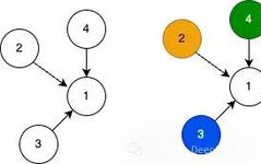
Below are shown two types of graphs: a homogeneous graph with the same node types and a heterogeneous graph with different node types connected. But what makes one node type different from another? The answer is simple: features! On the left is a homogeneous network, and on the right is a heterogeneous network:
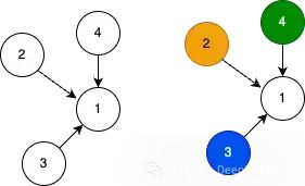
For the homogeneous graph, all features of nodes 1, 2, 3, and 4 have the same interpretation. For example, they all have two features, x and z, which I can compare between nodes. The edges within the network only connect nodes of the same type. For the heterogeneous graph, we also depict nodes 1, 2, 3, and 4 with similar connections, but in this case, each node type is unique, as shown by the colors.
This means that the features of node 1 are incompatible with those of nodes 2, 3, and 4. The simplest example is when the feature dimensions of node 1 differ from those of nodes 2, 3, and 4.
Many real-world systems are heterogeneous. For example, authors co-author papers that are published at conferences. For author nodes, information such as names and university affiliations may be stored; for papers, titles and abstracts are stored; and for conferences, names, addresses, and related information are stored. When a group of authors co-author a paper published at a specific conference, there will be links. However, features of the same node type are comparable, while features of different node types are not.
So first, we need to know how to store information for homogeneous networks and heterogeneous networks.
Data
We generate synthetic data to demonstrate how MessagePassing handles heterogeneous data structures.
Homogeneous Data
We generate some synthetic data for the network described above. For a homogeneous network, there are four nodes and a single node type; thus, all nodes have the same feature dimensions. We store the data in a single tensor as follows:
x = torch.tensor([[0.1234, 0.2345], [0.2303, -0.1863], [-1.1229, -0.6380], [2.2082, 0.7080]])
The edge index, which describes the connections, is defined as follows:
edge_index = torch.tensor([[1, 2, 3], [0, 0, 0]])
Here we only include edges pointing to node 1 (index 0).
Heterogeneous Data
In the definition of heterogeneous data, each data type has different dimensions. We create different feature sets, i.e., different feature dimensions. In the example graph, there are four unique types:
- A (node 1): feature dimension 2
- B (node 2): feature dimension 3
- C (node 3): feature dimension 4
-
D (node 4): feature dimension 5
Because each node type has different dimensions, we must store them in separate tensors. Here are the node features for nodes 1, 2, 3, and 4:
Node 1 features, dimension 2:
x_1 = torch.tensor([[0.1234, 0.2345]])
Node 2 features, dimension 3:
x_2 = torch.tensor([[0.2303, -0.1863, 0.5213]])
Node 3 features, dimension 4:
x_3 = torch.tensor([[-1.1229, -0.6380, 0.8640, 0.1297]])
Node 4 features, dimension 5:
x_4 = torch.tensor([[2.2082, 0.7080, -0.9620, 0.1297, 0.3769]])
Next is the MessagePassing algorithm.
Message Passing
Convolution layers are an extension of the MessagePassing algorithm. Here, we only discuss one important part – the computational graph – without going into too much detail. This computational graph is different from the network we study! Messages are sent from source nodes to target nodes, but multiple transformations occur before the final aggregated message reaches the target node. The diagram below illustrates this.
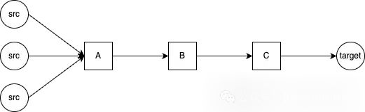
Illustrative representation of the computational graph
Below is a high-level overview of each transformation box:
- Aggregator A: Aggregates information from the same source node type. Available aggregation options are “sum”, “mean”, “min”, “max”, or “mul”.
- Projector B (SAGEConv layer): Linear projection that unifies the dimensions of various source node types.
-
Aggregator C: Aggregates information from the same target node type. Available aggregation options include “sum”, “mean”, “min”, “max”, “cat”, [None], with the default being “sum”.
Aggregator A is part of the MessagePassing algorithm; messages are aggregated according to the chosen aggregation scheme.
Projector B is part of the SAGEConv layer; to use the heterogeneous layer, it must utilize conv layers that support the OptPairTensor type. In other words, it must be able to accept different source and target node types. Other PYG layers that support this include GATConv and PPFConv.
Aggregator C is part of the HeteroConv layer; all aggregated messages from A are collected and combined into a feature vector for each node type.
Computational Graph of Homogeneous Networks
In the first example, we created a dataset with homogeneous data:
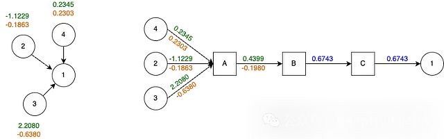
The computational graph of the homogeneous network (left) and the information propagating from the source node to target node 1 (right).
This computational graph updates the value of node 1. Messages from nodes 2, 3, and 4 are sent to node 1. Because the source nodes are of the same type, aggregator A aggregates all features by taking the average.
- 0.4399 = (0.2345 – 1.1229 + 2.2082) / 3
-
-0.1980 = (0.2303 – 0.1863 – 0.6380) / 3
Projector B transforms the feature vector [0.4399, -0.1980] into a one-dimensional vector 0.6743 through a linear layer. Here, the one-dimensional is arbitrary; it can be any dimension set. Additionally, the way SAGEConv implements the OptPairTensor may differ from other layers.
Aggregator C in the HeteroConv layer collects all messages sent to node 1, regardless of type. Thus, the final result is only of one type. Aggregator C passes the original message 0.6743 to node 1.
Computational Graph of Heterogeneous Networks
In the second data example, we stored the same data in a way that makes each node type unique.
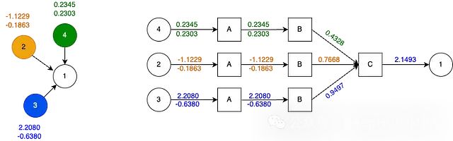
The computational graph of the heterogeneous network (left) and the information propagating from the source node to target node 1 (right).
There are three aggregators A because there are three different node types – nodes 2, 3, and 4 are unique! Aggregator A takes the average of individual messages and passes it to the linear projector B.
There are three linear projectors, one for each node type. The way projector B works is similar to before; it projects the 2D vector into a 1D vector.
Aggregator C collects all messages targeting node 1. It receives three messages, one from each unique source node type. Aggregator C sums the values of the incoming messages and passes them to node 1.
It can be seen that the same data yields completely different results!
In the last dataset, we added multiple nodes for each node type and connected them to node 1. This resulted in a computational graph where multiple nodes are aggregated by aggregator A before being sent to the linear projection layer. The diagram below shows the computational graph of this dataset:
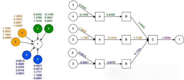
The computational graph of the heterogeneous network (left) and the information propagating from the source node to target node 1 (right). Only the first feature of each node type is shown in the computational graph.
It can be seen that aggregator A aggregates the feature information of the same node type. But essentially we have three homogeneous datasets and aggregators. After the projection layer, the features again become homogeneous datasets aggregated by C. This design of the computational graph allows us to aggregate feature information from heterogeneous nodes in the graph.
Conclusion
This is the complete process of message passing in heterogeneous graph neural networks. By understanding how messages are processed in the computational graphs of different datasets, we can gain deeper insights into how graph neural networks work. Applying these concepts to data can reveal the powerful insights and patterns that heterogeneous graph neural networks have in uncovering complex, interconnected information.
Author: Marcel BoersmaEditor: Huang Jiyan
About Us
Data派THU, as a public account for data science, backed by the Tsinghua University Big Data Research Center, shares cutting-edge research dynamics in data science and big data technology innovation, continuously disseminating knowledge in data science, striving to build a platform for gathering data talents, and creating the strongest group in China’s big data.

Sina Weibo: @数据派THU
WeChat Video Account: 数据派THU
Today’s Headlines: 数据派THU