Click on the above “Beginner Learning Vision”, select to add “Star” or “Top”
Heavyweight content delivered at the first time
Author: william
Link: https://zhuanlan.zhihu.com/p/133301967
This article is for sharing only, please delete if infringing
Feature extraction and matching is an important task in many computer vision applications, widely used in motion structure, image retrieval, object detection, and other fields. The feature detector that every beginner in computer vision learns about first is almost the HARRIS published in 1988. Over the decades, various feature detectors/descriptors have emerged like bamboo shoots after a rain, improving the accuracy and speed of feature detection.
Feature extraction and matching consist of three steps: keypoint detection, keypoint feature description, and keypoint matching. The combinations of different detectors, descriptors, and matchers are often confusing for beginners. This article will mainly introduce the principles behind keypoint detection, description, and matching, the advantages and disadvantages of different combinations, and propose several optimal combinations based on practical results.
Feature Extraction and Matching
Feature
A feature is information related to the computational task associated with solving a particular application. Features may be specific structures in an image, such as points, edges, or objects. Features can also be the results of general neighborhood operations or feature detection applied to images. These features can be divided into two main categories:
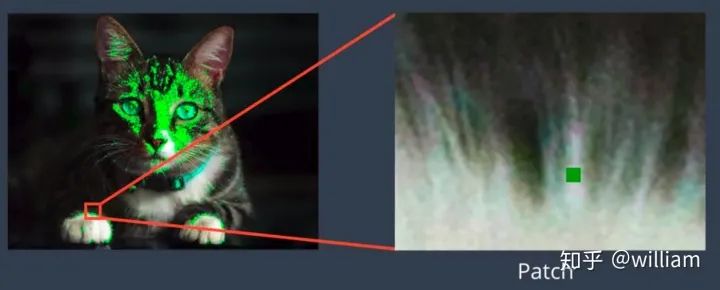
1. Features at specific locations in the image, such as peaks, building corners, doorways, or interestingly shaped snow blocks. These localized features are often referred to as keypoint features (or even corner points), and they are typically described by pixel blocks that appear around the point location, which is often referred to as an image patch.
2. Features that can be matched based on their direction and local appearance (edge contours) are called edges; they can also indicate object boundaries and occlusion events well in image sequences.
Main Components of Feature Extraction and Matching
1. Detection: Identifying interest points.
2. Description: Describing the local appearance around each feature point; this description is ideally invariant to changes in illumination, translation, scale, and planar rotation. We typically provide a descriptor vector for each feature point.
3. Matching: Identifying similar features by comparing descriptors in the images. For two images, we can obtain a set of pairs (Xi, Yi) -> (Xi’, Yi’), where (Xi, Yi) are the features of one image, and (Xi’, Yi’) are the features of another image.
Keypoints / Interest Points
Keypoints, also known as interest points, are points expressed in the texture. Keypoints are often points where the direction of the object boundary changes suddenly or intersection points between two or more edge segments. They have a clear position in image space or are well-located. Even if local or global disturbances such as illumination and brightness changes exist in the image domain, keypoints remain stable and can be reliably computed repeatedly. In addition, they should provide effective detection.
There are two methods for computing keypoints:
1. Based on the image brightness (usually through image derivatives).
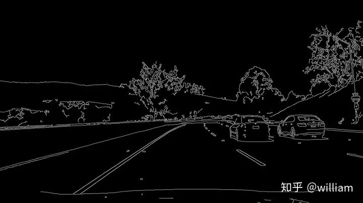
2. Based on boundary extraction (usually through edge detection and curvature analysis).
Invariance of Keypoint Detectors to Photometric and Geometric Changes
In the OPENCV library, we can choose from many feature detectors, and the choice of feature detector depends on the type of keypoints to be detected and the properties of the image, considering the robustness of the corresponding detector to photometric and geometric transformations.
When selecting an appropriate keypoint detector, we need to consider four basic transformation types:
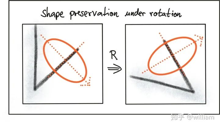
1. Rotation Transformation
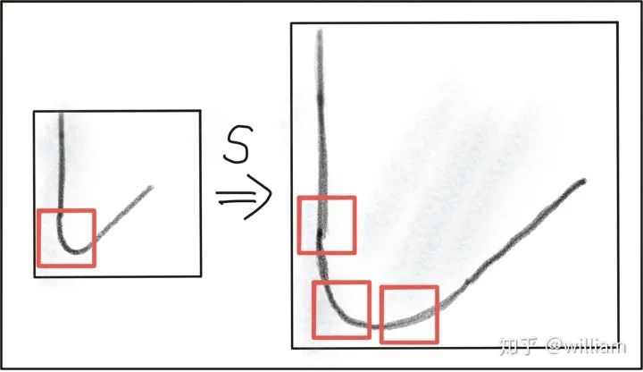
3. Intensity Transformation
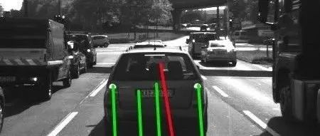
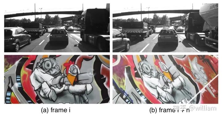
The graffiti sequence is one of the standard image sets used in computer vision, and we can observe that the graffiti image at frame i+n includes all transformation types. For the highway sequence, when focusing on the vehicles in front, there are only scale and intensity changes between frame i and frame i+n.
The traditional HARRIS sensor is robust to rotation and additive intensity offset but sensitive to scale changes, multiplicative intensity offset (i.e., contrast changes), and affine transformations.
Automatic Scale Selection
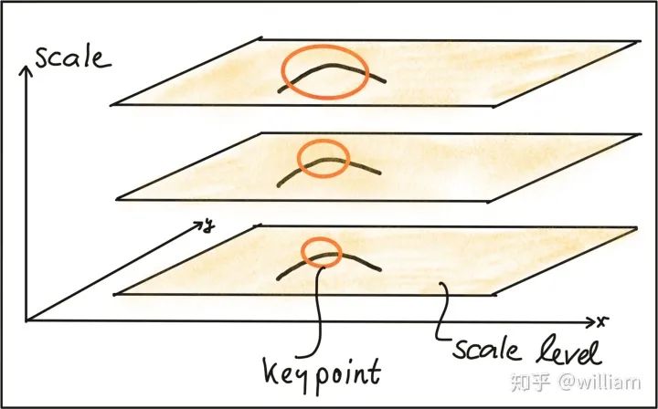
To detect keypoints at the ideal scale, we must know (or find) their respective dimensions in the image and adapt the size of the Gaussian window w(x,y) introduced in the previous section. If the scale of the keypoints is unknown or if the keypoints exist in images of different sizes, detection must be performed continuously at multiple scale levels.
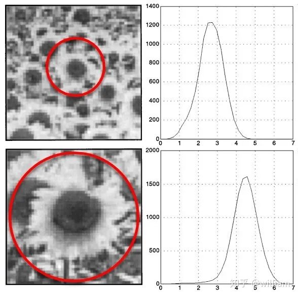
Based on the standard deviation increment between adjacent layers, the same keypoint may be detected multiple times. This raises the question of selecting the “correct” scale that best represents the keypoint. In 1998, Tony Lindeberg published a method called “Feature Detection with Automatic Scale Selection.” It proposed a function f(x,y,scale) that can be used to select keypoints that have stable maxima at the scale FF. The scale at which Ff is maximized is referred to as the “feature scale” of each keypoint.
As shown in the figure below, such a function FF has been evaluated over several scale levels, and the second image shows a clear maximum that can be viewed as the feature scale of the image content within a circular area.
A good detector can automatically select the feature scale of keypoints based on the structural characteristics of the local neighborhood. Modern keypoint detectors typically have this capability, thus being highly robust to changes in image scale.
Common Keypoint Detectors
Keypoint detectors are a very popular research area, and many powerful algorithms have been developed over the years. Applications of keypoint detection include object recognition and tracking, image matching and panorama stitching, as well as robotic mapping and 3D modeling. The choice of detector not only needs to compare the invariance in the transformations mentioned above but also needs to compare the detection performance and processing speed of the detectors.
Classic Keypoint Detectors
The purpose of classic keypoint detectors is to maximize detection accuracy, and complexity is generally not the primary concern.
HARRIS– 1988 Harris Corner Detector (Harris, Stephens)
Shi, Tomasi– 1996 Good Features to Track (Shi, Tomasi)
SIFT– 1999 Scale Invariant Feature Transform (Lowe) – None free
SURF– 2006 Speeded Up Robust Features (Bay, Tuytelaars, Van Gool) – None free
Modern Keypoint Detectors
In recent years, some faster detectors have been developed for real-time applications on smartphones and other portable devices. The list below shows the most popular detectors in this group:
FAST– 2006 Features from Accelerated Segment Test (FAST) (Rosten, Drummond)
BRIEF– 2010 Binary Robust Independent Elementary Features (BRIEF) (Calonder, et al.)
ORB– 2011 Oriented FAST and Rotated BRIEF (ORB) (Rublee et al.)
BRISK– 2011 Binary Robust Invariant Scalable Keypoints (BRISK) (Leutenegger, Chli, Siegwart)
FREAK– 2012 Fast Retina Keypoint (FREAK) (Alahi, Ortiz, Vandergheynst)
KAZE– 2012 KAZE (Alcantarilla, Bartoli, Davidson)
Gradient and Binary-based Descriptors
Since our task is to find corresponding keypoints in image sequences, we need a method based on similarity measures to reliably assign keypoints to each other. Various similarity measures (called Descriptors) have been proposed in the literature, and many authors have simultaneously published a new method for keypoint detection optimized for their keypoint types. In other words, the encapsulated OPENCV keypoint detector functions can mostly be used to generate keypoint descriptors as well.
Keypoint detectors are algorithms that select points from images based on local maxima of functions, such as the “corner” measures we see in the HARRIS detector.
Keypoint descriptors are vectors used to describe the pixel values of the image patch around keypoints. Describing methods include comparing raw pixel values and more complex methods like histograms of gradient directions.
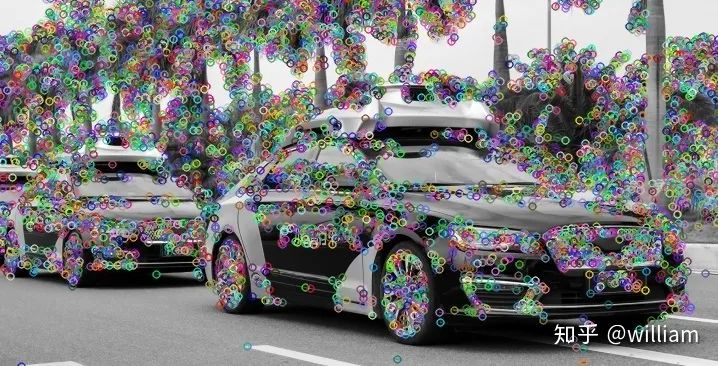
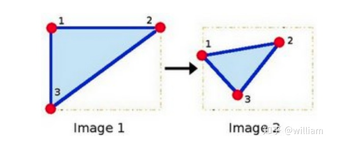
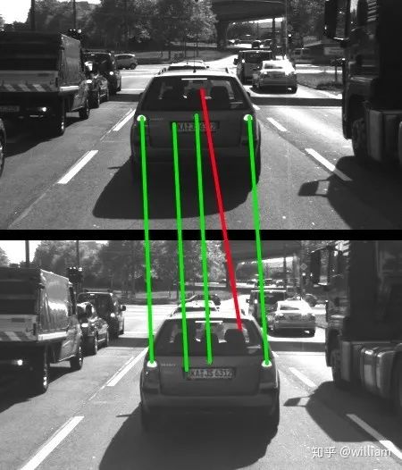
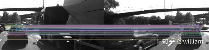
Keypoint detectors generally find feature points from a frame image. Descriptors help us assign similar keypoints from different images to each other in the “keypoint matching” step. As shown in the figure below, a set of keypoints in one frame is assigned to keypoints in another frame to maximize the similarity of their descriptors, and these keypoints represent the same object in the image. In addition to maximizing similarity, good descriptors should minimize mismatches, i.e., avoid assigning keypoints that do not correspond to the same object to each other.
HOG-based Descriptors
Although more and more fast detector/descriptor combinations have emerged, the scale-invariant feature transform (SIFT), based on histogram of oriented gradients (HOG), is still widely used. The basic idea of HOG is to describe the structure of objects by the distribution of intensity gradients in the local neighborhood of the object. To achieve this, the image is divided into several cells, where gradients are computed and collected into histograms. The histogram sets of all cells are then used as similarity measures to uniquely identify image blocks or objects.
SIFT/SURF uses HOG as descriptors, including both keypoint detectors and descriptors, which are powerful but patented. SURF is an improvement on SIFT, which not only increases computational speed but also enhances robustness. The implementation principles of the two are very similar. Here, I will only introduce SIFT.
The SIFT method follows a five-step process, which will be briefly summarized below.
First, keypoints in the image are detected using a method called “Laplacian of Gaussian (LoG),” which is based on the second-order intensity derivatives. LoG is applied at various scale levels of the image and tends to detect blobs rather than corners. In addition to using a unique scale level, directions are assigned to keypoints based on the intensity gradients in the local neighborhood around the keypoint.
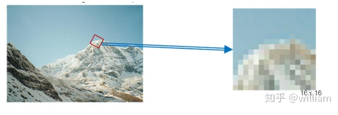
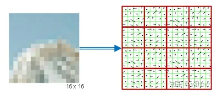
Second, for each keypoint, the surrounding area is altered by eliminating the direction, thus ensuring a standardized direction. Moreover, the size of the area is adjusted to 16 x 16 pixels, providing a standardized image patch.
Third, the direction and magnitude of each pixel in the normalized image patch are computed based on intensity gradients _Ix_ and _Iy_.
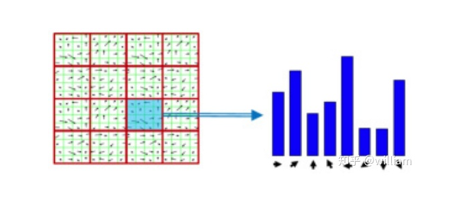
Fourth, the normalized patch is divided into a grid of 4 x 4 cells. Within each cell, the directions of pixels exceeding the magnitude threshold are collected in a histogram consisting of 8 bins.
Finally, all 16 cell histograms of 8 bars are concatenated into a 128-dimensional vector (descriptor) that uniquely represents the keypoint.
SIFT detectors/descriptors can reliably identify objects even in clutter and partial occlusions. Uniform changes in scale, rotation, brightness, and contrast are invariant, and affine distortions are even invariant.
The disadvantage of SIFT is its low speed, which makes it unsuitable for real-time applications on devices like smartphones. Other members of the HOG series (such as SURF and GLOH) have been optimized for speed. However, they are still computationally expensive and should not be used in real-time applications. Moreover, SIFT and SURF have numerous patents, so they cannot be freely used in commercial environments. To use SIFT in OpenCV, you must include #include <opencv2/xfeatures2d/nonfree.hpp> and install the OPENCV_contribute package, ensuring that OPENCV_ENABLE_NONFREE is enabled in the CMake options.
The issue with HOG-based descriptors is that they rely on computing intensity gradients, which is a very expensive operation. Even though some improvements have been made (e.g., SURF uses integral images for speedup), these methods are still not suitable for real-time applications on devices with limited processing power (e.g., smartphones). The family of binary descriptors provides a faster (and free) alternative to HOG-based methods, albeit with slightly lower accuracy and performance.
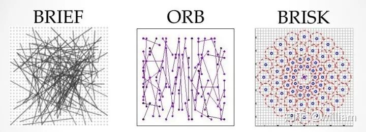
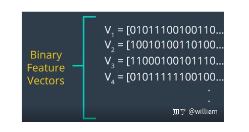
The core idea of binary descriptors is to rely solely on intensity information (i.e., the image itself) and encode information around keypoints into a string of binary numbers, which can be compared very efficiently during the matching step. In other words, binary descriptors encode information about interest points into a series of numbers and serve as a digital “fingerprint” to distinguish one feature from another. Currently, the most popular binary descriptors are BRIEF, BRISK, ORB, FREAK, and KAZE (all of which can be found in the OpenCV library).
From a high-level perspective, binary descriptors consist of three main parts:
1. A sampling pattern that describes the positions of sample points around the keypoint.
2. A direction compensation method that eliminates the influence of rotation around the keypoint location.
3. A method for selecting sample pairs that generates paired sample points, which are compared based on their intensity values. If the first value is greater than the second value, we write a “1” in the binary string; otherwise, we write a “0.” After performing this operation on all pairs of points in the sampling pattern, a long binary chain (or “string”) is created (hence the name of the descriptor class family).
BRISK “Binary Robust Invariant Scalable Keypoints” is a representative keypoint detector/descriptor. Here, I will only introduce BRISK.
In 2011, Stefan Leutenegger proposed BRISK, a combination of a FAST detector and a Binary Descriptor created by intensity comparisons obtained through specialized sampling of each keypoint’s neighborhood.
The sampling pattern of BRISK consists of multiple sampling points (in blue), where concentric rings (in red) around each sampling point indicate the areas where Gaussian smoothing is applied. Unlike some other binary descriptors (e.g., ORB or Brief), the BRISK sampling pattern is fixed. Smoothing is crucial to avoid aliasing (an effect that makes it difficult to distinguish between different signals when sampled – or to blend them together).
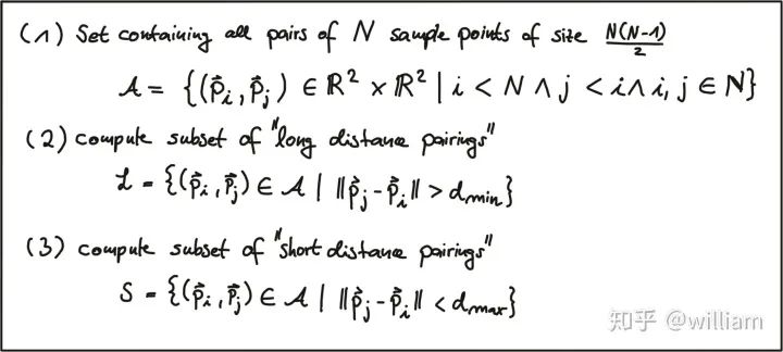
During the sample pair selection, the BRISK algorithm distinguishes between long-distance and short-distance pairs. Long-distance pairs (i.e., sample points that have the minimum distance from each other in the sampling pattern) are used to estimate the direction of the image patch based on intensity gradients, while short-distance pairs are used to perform intensity comparisons on the assembled descriptor string. Mathematically, these pairs are represented as follows:
First, we define the set A of all possible pairs of sampling points. Then, we extract the subset L from A, where the Euclidean distance of subset L is above a certain threshold. L is used for direction estimation with long-distance pairs. Finally, we extract those pairs from A whose Euclidean distance is below a lower threshold. This set S contains short-distance pairs used to assemble the binary descriptor string.
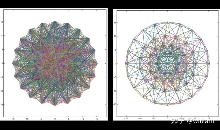
The figure below shows the two types of distance pairs on the sampling pattern: short pairs (left) and long pairs (right).
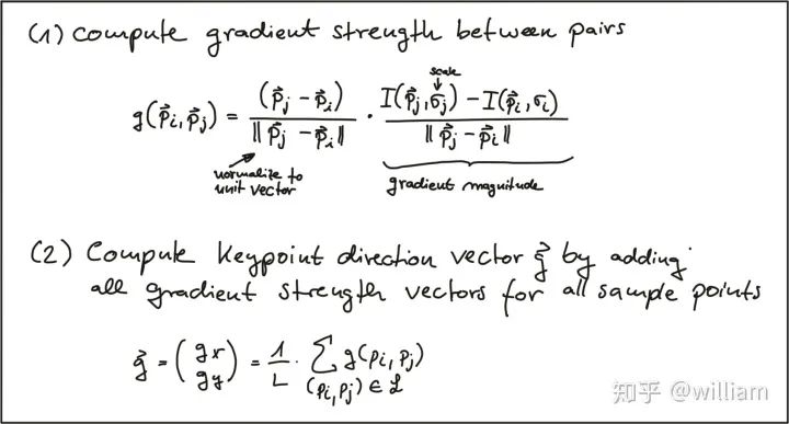
From the long pairs, the keypoint direction vector G is computed as follows:
First, the gradient intensity between the two sampling points is computed based on normalized unit vectors, where the normalized unit vector provides the direction between the two points, multiplied by the intensity difference between the two points at their respective scales. Then, in (2), the keypoint direction vector g is calculated from the total of all gradient intensities.
Based on g, we can rearrange the short-distance pairs using the direction of the sampling pattern to ensure rotational invariance. Based on the rotation-invariant short-distance pairs, the final binary descriptor can be constructed as follows:
OPENCV Detector/Descriptor Implementation
Currently, there are various feature point detectors/descriptors, such as HARRIS, SHI-TOMASI, FAST, BRISK, ORB, AKAZE, SIFT, FREAK, and BRIEF. Each of these deserves a blog post of its own, but the purpose of this article is to provide an overview, so I will not analyze these detectors/descriptors in detail from a theoretical perspective. There are numerous articles online describing these detectors/descriptors, but I still recommend that you first check out OPENCV’s Tutorial: How to Detect and Track Object With OpenCV.
Below, I will introduce the code implementation and parameter details for each feature point detector/descriptor, and at the end of the article, I will evaluate these combinations based on practical results.
Some OPENCV functions can be used for both detectors/descriptors, but some combinations may have issues.
SIFT Detector/Descriptor SIFT detector and ORB descriptor do not work together
int nfeatures = 0;// The number of best features to retain.int nOctaveLayers = 3;// The number of layers in each octave. 3 is the value used in D. Lowe paper.double contrastThreshold = 0.04;// The contrast threshold used to filter out weak features in semi-uniform (low-contrast) regions. double edgeThreshold = 10;// The threshold used to filter out edge-like features. double sigma = 1.6; // The sigma of the Gaussian applied to the input image at the octave #0.xxx=cv::xfeatures2d::SIFT::create(nfeatures, nOctaveLayers, contrastThreshold, edgeThreshold, sigma);
// Detector parametersint blockSize = 2; // for every pixel, a blockSize × blockSize neighborhood is consideredint apertureSize = 3; // aperture parameter for Sobel operator (must be odd)int minResponse = 100; // minimum value for a corner in the 8bit scaled response matrixdouble k = 0.04; // Harris parameter (see equation for details)// Detect Harris corners and normalize outputcv::Mat dst, dst_norm, dst_norm_scaled;dst = cv::Mat::zeros(img.size(), CV_32FC1);cv::cornerHarris(img, dst, blockSize, apertureSize, k, cv::BORDER_DEFAULT);cv::normalize(dst, dst_norm, 0, 255, cv::NORM_MINMAX, CV_32FC1, cv::Mat());cv::convertScaleAbs(dst_norm, dst_norm_scaled);// Look for prominent corners and instantiate keypointsdouble maxOverlap = 0.0; // max. permissible overlap between two features in %, used during non-maxima suppressionfor (size_t j = 0; j < dst_norm.rows; j++) { for (size_t i = 0; i < dst_norm.cols; i++) { int response = (int) dst_norm.at<float>(j, i); if (response > minResponse) { // only store points above a threshold cv::KeyPoint newKeyPoint; newKeyPoint.pt = cv::Point2f(i, j); newKeyPoint.size = 2 * apertureSize; newKeyPoint.response = response; // perform non-maximum suppression (NMS) in local neighbourhood around new key point bool bOverlap = false; for (auto it = keypoints.begin(); it != keypoints.end(); ++it) { double kptOverlap = cv::KeyPoint::overlap(newKeyPoint, *it); if (kptOverlap > maxOverlap) { bOverlap = true; if (newKeyPoint.response > (*it).response) { // if overlap is >t AND response is higher for new kpt *it = newKeyPoint; // replace old key point with new one break; // quit loop over keypoints } } } if (!bOverlap) { // only add new key point if no overlap has been found in previous NMS keypoints.push_back(newKeyPoint); // store new keypoint in dynamic list } } } // eof loop over cols} // eof loop over rows
SHI-TOMASI Detector
int blockSize = 6; // size of an average block for computing a derivative covariation matrix over each pixel neighborhooddouble maxOverlap = 0.0; // max. permissible overlap between two features in %double minDistance = (1.0 - maxOverlap) * blockSize;int maxCorners = img.rows * img.cols / max(1.0, minDistance); // max. num. of keypointsdouble qualityLevel = 0.01; // minimal accepted quality of image cornersdouble k = 0.04;bool useHarris = false;// Apply corner detectionvector<cv::Point2f> corners;cv::goodFeaturesToTrack(img, corners, maxCorners, qualityLevel, minDistance, cv::Mat(), blockSize, useHarris, k);// add corners to result vectorfor (auto it = corners.begin(); it != corners.end(); ++it) { cv::KeyPoint newKeyPoint; newKeyPoint.pt = cv::Point2f((*it).x, (*it).y); newKeyPoint.size = blockSize; keypoints.push_back(newKeyPoint);}
BRISK Detector/Descriptor
int threshold = 30; // FAST/AGAST detection threshold score.int octaves = 3; // detection octaves (use 0 to do single scale)float patternScale = 1.0f; // apply this scale to the pattern used for sampling the neighbourhood of a keypoint.xxx=cv::BRISK::create(threshold, octaves, patternScale);
FREAK Detector/Descriptor
bool orientationNormalized = true;// Enable orientation normalization.bool scaleNormalized = true;// Enable scale normalization.float patternScale = 22.0f;// Scaling of the description pattern.int nOctaves = 4;// Number of octaves covered by the detected keypoints.const std::vector<int> &selectedPairs = std::vector<int>(); // (Optional) user defined selected pairs indexes,xxx=cv::xfeatures2d::FREAK::create(orientationNormalized, scaleNormalized, patternScale, nOctaves,selectedPairs);
int threshold = 30;// Difference between intensity of the central pixel and pixels of a circle around this pixelbool nonmaxSuppression = true;// perform non-maxima suppression on keypointscv::FastFeatureDetector::DetectorType type = cv::FastFeatureDetector::TYPE_9_16;// TYPE_9_16, TYPE_7_12, TYPE_5_8xxx=cv::FastFeatureDetector::create(threshold, nonmaxSuppression, type);
ORB Detector/Descriptor SIFT detector and ORB descriptor do not work together
int nfeatures = 500;// The maximum number of features to retain.float scaleFactor = 1.2f;// Pyramid decimation ratio, greater than 1.int nlevels = 8;// The number of pyramid levels.int edgeThreshold = 31;// This is size of the border where the features are not detected.int firstLevel = 0;// The level of pyramid to put source image to.int WTA_K = 2;// The number of points that produce each element of the oriented BRIEF descriptor.auto scoreType = cv::ORB::HARRIS_SCORE;// The default HARRIS_SCORE means that Harris algorithm is used to rank features.int patchSize = 31;// Size of the patch used by the oriented BRIEF descriptor.int fastThreshold = 20;// The fast threshold.xxx=cv::ORB::create(nfeatures, scaleFactor, nlevels, edgeThreshold, firstLevel, WTA_K, scoreType,patchSize, fastThreshold);
AKAZE Detector/Descriptor KAZE/AKAZE descriptors will only work with KAZE/AKAZE detectors.
auto descriptor_type = cv::AKAZE::DESCRIPTOR_MLDB;// Type of the extracted descriptor: DESCRIPTOR_KAZE, DESCRIPTOR_KAZE_UPRIGHT, DESCRIPTOR_MLDB or DESCRIPTOR_MLDB_UPRIGHT.int descriptor_size = 0;// Size of the descriptor in bits. 0 -> Full sizeint descriptor_channels = 3;// Number of channels in the descriptor (1, 2, 3)float threshold = 0.001f;// Detector response threshold to accept pointint nOctaves = 4;// Maximum octave evolution of the imageint nOctaveLayers = 4;// Default number of sublevels per scale levelauto diffusivity = cv::KAZE::DIFF_PM_G2;// Diffusivity type. DIFF_PM_G1, DIFF_PM_G2, DIFF_WEICKERT or DIFF_CHARBONNIERxxx=cv::AKAZE::create(descriptor_type, descriptor_size, descriptor_channels, threshold, nOctaves,nOctaveLayers, diffusivity);
BRIEF Detector/Descriptor
int bytes = 32;// Length of the descriptor in bytes, valid values are: 16, 32 (default) or 64 .bool use_orientation = false;// Sample patterns using keypoints orientation, disabled by default.xxx=cv::xfeatures2d::BriefDescriptorExtractor::create(bytes, use_orientation);
Feature matching or image matching in general is part of computer vision applications such as image registration, camera calibration, and object recognition, which involves establishing correspondences between two images of the same scene/target. A commonly used image matching method detects a set of interest points associated with image descriptors from image data. Once features and descriptors have been extracted from two or more images, the next step is to establish some preliminary feature matches between these images.
Generally, the performance of feature matching methods depends on the nature of the underlying keypoints and the selection of the corresponding image descriptors.
We have learned that keypoints can be described by transforming their local neighborhoods into high-dimensional vectors that capture unique characteristics of the gradient or intensity distribution.
Distance Between Descriptors
Feature matching requires calculating the distance between two descriptors, so their differences are converted into a single number that can be used as a simple similarity measure.
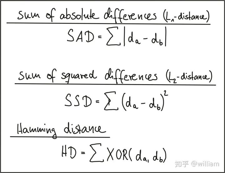
Currently, there are three distance metrics:
-
Sum of Absolute Differences (SAD) – L1-norm
-
Sum of Squared Differences (SSD) – L2-norm
-
The difference between SAD and SSD is that the shortest distance between the two is a straight line. Given the two components of each vector, SAD computes the sum of length differences, which is a one-dimensional process. SSD, on the other hand, computes the sum of squares, following the Pythagorean theorem; in a rectangular triangle, the sum of squares of the width equals the square of the hypotenuse. Therefore, in terms of geometric distance between two vectors, L2-norm is a more accurate measure. Note that the same principle applies to high-dimensional descriptors.
Hamming distance is suitable for binary descriptors consisting only of 1s and 0s, calculated by using the XOR function to compute the differences between two vectors; if two bits are the same, it returns zero, and if they differ, it returns one. Thus, the total sum of all XOR operations is the number of differing bits between the two descriptors.
It is important to select the appropriate distance metric based on the type of descriptor used.
-
BINARY descriptors: BRISK, BRIEF, ORB, FREAK, and AKAZE – Hamming distance
-
HOG descriptors: SIFT (and SURF and GLOH, all patented) – L2-norm
Finding Matching Pairs
Let’s assume there are N keypoints and their associated descriptors in one image and M keypoints in another image.
Brute Force Matching
The most straightforward way to find corresponding pairs is to compare all features against each other, performing N x M comparisons. For a given keypoint in the first image, it will take each keypoint from the second image and calculate the distance. The keypoint with the smallest distance will be considered a match. This method is called “Brute Force Matching” or “Nearest Neighbor Matching.” The output of brute-force matching in OPENCV is a list of keypoint pairs sorted by their descriptor distances under the selected distance function.
Fast Nearest Neighbor (FLANN)
In 2014, David Lowe and Marius Muja released