Source: DeepHub IMBA

This article is approximately 3400 words and is recommended for a 7-minute read.
This article introduces the theoretical basis for finding similar images and uses a system for trademark search as an example to introduce the relevant technical implementation.
This article will introduce the theoretical basis for finding similar images and uses a system for trademark search as an example to introduce the relevant technical implementation. It provides background information on recommended methods used in image retrieval tasks. After reading this article, you will be able to create an image search engine from scratch.
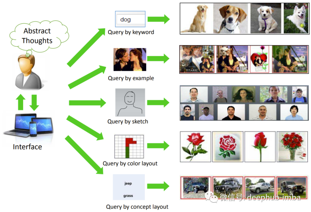
Image retrieval (also known as Content-Based Image Retrieval or CBIR) is the foundation of any search involving images.
The above image is from the article Recent Advance in Content-based Image Retrieval: A Literature Survey (2017) arxiv:1706.06064
The “search by image” method has appeared in various fields, especially on e-commerce websites (e.g., Taobao), and the “search images by keywords” (understanding image content) has long been used by search engines like Google, Baidu, Bing, etc. I believe that since the emergence of the groundbreaking CLIP: Connecting Text and Images in the computer vision community, the globalization of this method will accelerate.
This article will only discuss image search methods based on neural networks in computer vision research.
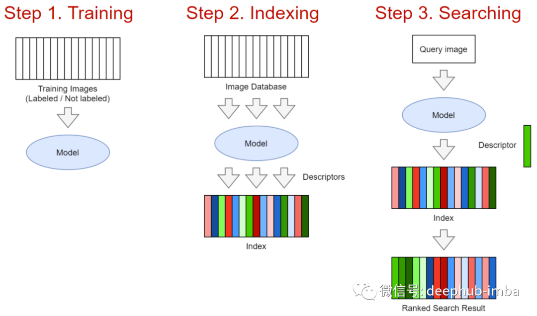
Basic Service Components
Step 1. Train the model. The model can be created based on classical CV or neural network. Model input – image, output – D-dimensional feature embedding. In traditional cases, it can be a combination of SIFT descriptor + Bag of Visual Words. In the case of neural networks, it can be standard backbones like ResNet, EfficientNet, etc., plus complex pooling layers. If there is enough data, neural networks almost always perform well, so we will focus on them.
Step 2. Index images. Indexing is the process of running the trained model on all images and writing the obtained embeddings into a special index for quick search.
Step 3. Search. Using the user-uploaded image, obtain the embedding through the model, and compare that embedding with the embeddings of other images in the database (index), and the search results can be sorted by relevance.
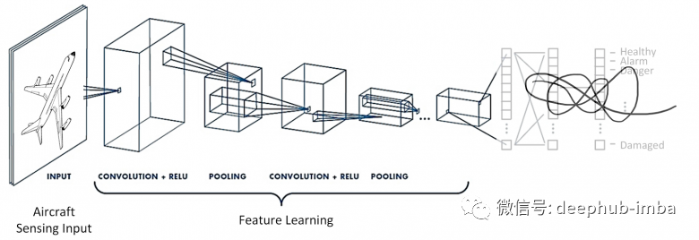
Neural Networks and Metric Learning
In similarity search tasks, the role of neural networks is as feature extractors (backbone networks). The choice of backbone network depends on the quantity and complexity of the data – models from ResNet18 to Visual Transformer can be considered.
The first characteristic of models in image retrieval is the design of the neural network head. On the Image Retrieval leaderboard (https://kobiso.github.io/Computer-Vision-Leaderboard/cars.html), they can achieve optimal image feature descriptions that make the activation distribution of output feature maps more uniform through techniques like parallel pools, Batch Drop Block, etc.
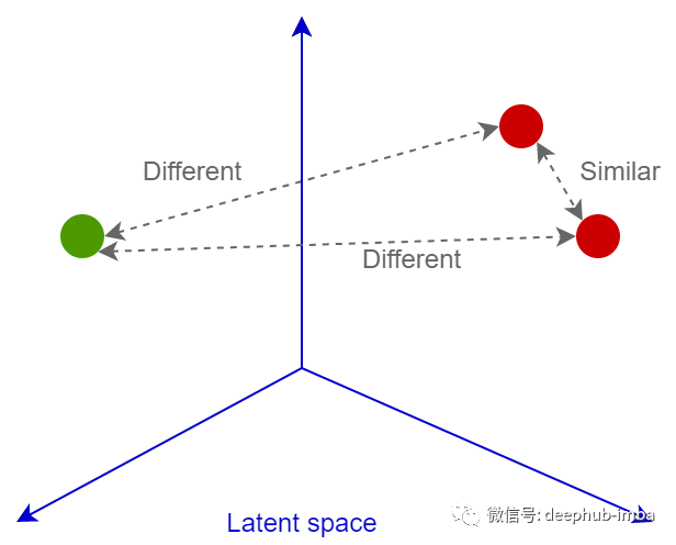
The second main feature is the selection of the loss function. In the Deep Image Retrieval: A Survey (arxiv 2101.11282), there are dozens of recommended loss functions that can be used for pairwise training. The main purpose of all these losses is to train the neural network to convert images into vectors in a linearly separable space, so that these vectors can be compared further by cosine or Euclidean distance: similar images will have close embeddings, while dissimilar images will be relatively far apart. Let’s take a look at several main loss functions.
Loss Functions
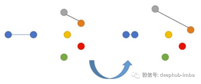
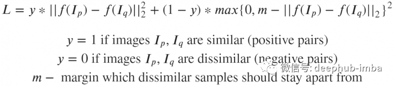
This is a dual loss, where objects are compared based on their distances from each other.
If these images are indeed similar, the neural network will be penalized for the distance between the embeddings of images p and q being too far apart. If the images are actually different but the embeddings are close together, it will also be penalized, but in this case, a margin m (for example, 0.5) is set, which assumes that the neural network has already dealt with the task of “separating” different images and does not need excessive punishment.
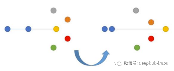
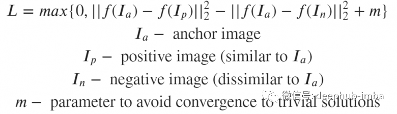
The goal of this loss is to minimize the distance from the anchor to the positive and maximize the distance from the anchor to the negative. Triplet Loss was first introduced in Google’s FaceNet paper on face recognition and has long been a state-of-the-art solution.
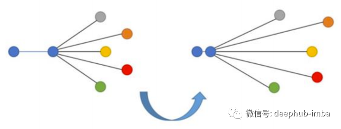
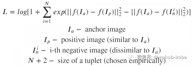
N-tupled Loss is a development of Triplet Loss, which also uses anchor and positive but employs multiple negative samples instead of one.
4. Angular Additive Margin (ArcFace)
The problem with dual loss is the choice of combinations of anchor, positive, and negative – if they are just evenly randomly sampled from the dataset, the “light pairs” problem will occur, where the loss for certain image pairs will be 0, causing the network to converge very quickly to a state because most of the sample pairs in our input are very “easy” for it, and when the loss is 0, the network stops learning. To avoid this problem, ArcFace proposes complex mining techniques for pairing samples – hard negative and hard positive mining. Interested parties can look at a library called PML, which implements many mining methods and contains a lot of useful information about Metric Learning tasks on PyTorch.
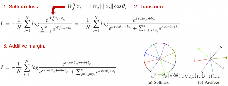 Another solution to the light pairs problem is classification loss. The main idea of ArcFace is to add an indentation m to the usual cross-entropy, which allows embeddings of similar images to distribute around the centroid area of that class, so they are all separated from the embeddings of other classes by the smallest angle m.
This is a perfect loss function, especially when benchmarking with MegaFace. However, ArcFace only works when there are classification labels. After all, if there are no classification labels, cross-entropy cannot be calculated, right?
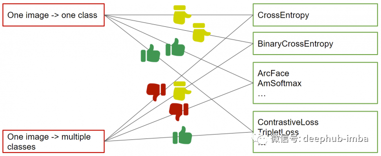
The above image shows recommendations for selecting loss functions with single-class and multi-class labels (if there are no labels, matching pairs can also be generated by calculating the percentage of intersection between the multi-label vectors of samples).
Another solution to the light pairs problem is classification loss. The main idea of ArcFace is to add an indentation m to the usual cross-entropy, which allows embeddings of similar images to distribute around the centroid area of that class, so they are all separated from the embeddings of other classes by the smallest angle m.
This is a perfect loss function, especially when benchmarking with MegaFace. However, ArcFace only works when there are classification labels. After all, if there are no classification labels, cross-entropy cannot be calculated, right?
The above image shows recommendations for selecting loss functions with single-class and multi-class labels (if there are no labels, matching pairs can also be generated by calculating the percentage of intersection between the multi-label vectors of samples).
Pooling
Pooling is also frequently used in neural network architectures, below are several pooling layers used in image retrieval tasks.
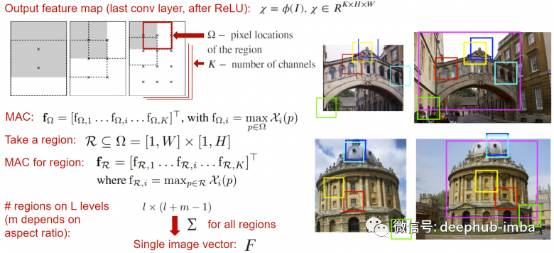
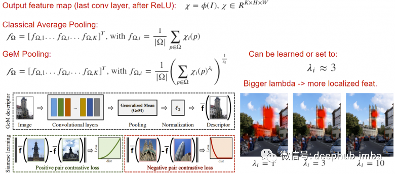
Regional Maximum Activation of Convolutions (R-MAC) can be seen as a pooling layer that takes the output feature maps from the neural network (before global pooling or classification layers) and returns a vector description of the total activation computed based on different windows, where the activation of each window is the maximum value taken independently for each channel.
This operation creates richer feature descriptions by constructing local features of the image at different scales. This descriptor itself is an embedded vector, so it can be directly fed into the loss function.
Generalized Mean (GeM) is a simple pooling operation that can improve the quality of output descriptors by applying the lambda norm to average pooling operations. By increasing lambda, the network focuses on the important parts of the image, which is effective in some tasks.
Distance Measurement
Another key point for high-quality similar image search is ranking, which displays the most relevant results for a given query. Its main metrics are the speed of indexing, the speed of searching, and the memory consumed.
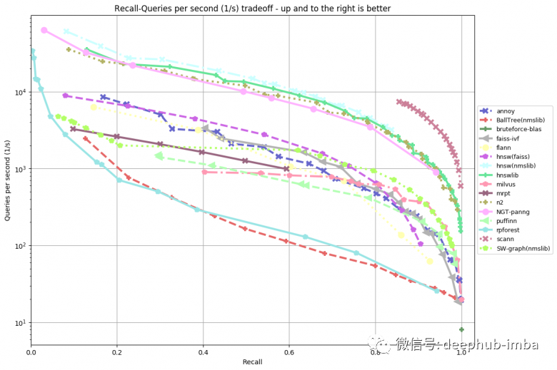
The simplest method is to perform a brute-force search directly using the embedding vectors, such as using cosine distance. However, when dealing with large amounts of data – millions, tens of millions, or even more – the search speed significantly decreases.
These problems can be solved at the cost of quality – by compressing (quantizing) rather than storing embeddings in their raw form. At the same time, the search strategy is also changed – instead of using brute force search, it attempts to find the closest embedding vector to the given query with the least number of comparisons. There are many efficient frameworks available for approximate nearest neighbor search, such as NMSLIB, Spotify Annoy, Facebook Faiss, and Google Scann. In addition to machine learning libraries, traditional Elasticsearch also supports vector queries after version 7.3.
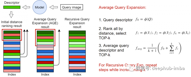
Researchers in the field of information retrieval have long discovered that after receiving the original search results, the quality of search results can be improved by reordering the collection in some way.
Using the top-k closest searches to generate new embeddings, in the simplest case, the average vector can be taken. As shown in the above image, embeddings can also be weighted, for example, by the distance in the query or weighted ranking by cosine distance with the request.
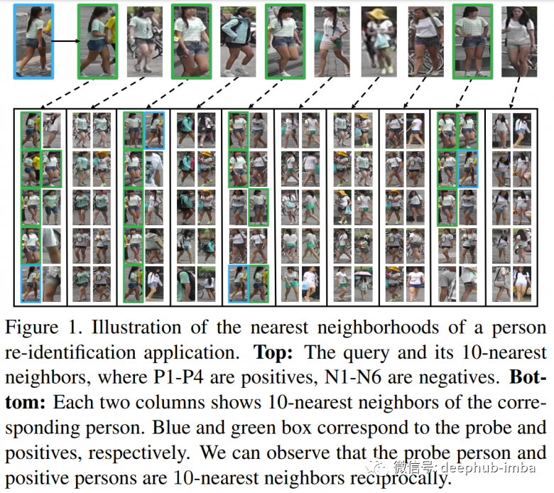
k-reciprocal is a set of elements from top-k that includes the k closest elements to the query itself, based on this set, a reordering process is constructed, one of which is described in the paper Re-ranking Person Re-identification with k-reciprocal Encoding. k-reciprocal is closer to the query than k nearest neighbors. Therefore, the elements concentrated in k-reciprocal can be roughly regarded as known positive samples, and the weighting rules can be changed. The original paper contains a lot of calculations that exceed the scope of this article, and interested readers are recommended to read it.
Validation Metrics
Finally, we check the quality of similar searches. Beginners may not notice many nuances in this task when they first start working on image retrieval projects.
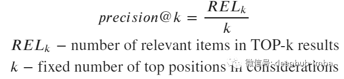
Let’s take a look at these popular metrics in image retrieval tasks: precision@k, recall@k, R-precision, mAP, and nDCG.
Advantages: Shows the percentage of relevant top-k.
-
Very sensitive to the number of relevant samples for a given query, which may produce a non-objective evaluation of search quality since different queries have different numbers of relevant results.
-
Can only reach 1 if the number of relevant samples for all queries >= k.
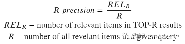
Same as precision@k, where k is set equal to the number of relevant queries.
Advantages: Eliminates sensitivity to the number k in precision@k, making the metric stable.
Disadvantages: Must know the total number of samples relevant to the query request (if not all relevant ones are tagged, it will cause problems).
Proportion of relevant items found in top-k.
-
This metric answers whether relevant results were found in top-k.
-
Can handle requests stably and on average.
4. mAP (mean Average Precision)
Density of relevant results filling the top of search results. It can be viewed as the number of pages that a search engine user needs to read when receiving the same amount of information (the fewer, the better).
Advantages: Objective and stable evaluation of retrieval quality.
Disadvantages: Must know the total number of samples relevant to the request.
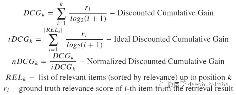
5. nDCG (Normalized Discounted Gain)
This metric shows whether the elements in top-k are correctly ranked among themselves. The advantages and disadvantages of this metric will not be introduced here, as it is the only metric in the list that considers the order of elements. Studies have shown that when order needs to be considered, this metric is quite stable and applicable in most cases.
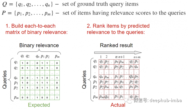
6. Recommended Validation Schemes
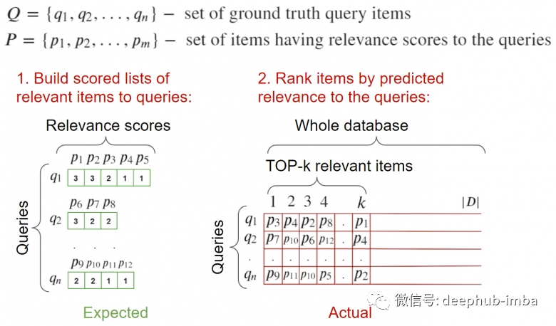
6a. Validate against a set of queries and selected relevant queries.
Input: Query image and images related to it. A list of tags related to this query is required.
To calculate metrics: Calculate the relevant matrix for each and compute metrics based on the relevance information of the elements.
6b. Full database validation.
Input: Query images and images related to them. Ideally, there should be a validation database for images, where all relevant queries are tagged. It should be noted that the query image should not be included in the relevant images to avoid it being ranked top-1; our task is to find relevant images, not to find the image itself.
To calculate metrics: Traverse all requests, calculate the distances to all elements (including relevant elements), and send them to the metric calculation function.
Complete Example Introduction
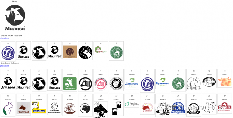
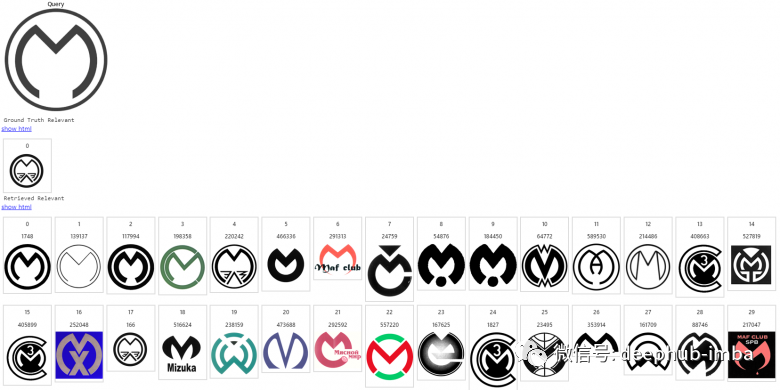
Here, we introduce how the image search engine works using the example of searching for similar trademark logos.
Size of the image index database: millions of trademarks. The first image here is a query, the next line is the list of relevant returns, and the remaining rows are the content provided by the search engine in descending order of relevance.
Conclusion
That’s it, I hope this article can provide a complete idea for those who are building or about to build a similar image search engine. If you have any good suggestions, feel free to leave a comment.