Extreme Gradient Boosting (XGBoost) Ensemble in Python

Extreme Gradient Boosting (XGBoost) is an open-source library that provides an efficient implementation of the gradient boosting algorithm.

Although other open-source implementations of this method existed before XGBoost, the release of XGBoost seems to have unleashed the power of the technique and brought gradient boosting to the attention of the machine learning community at large. Shortly after its development and initial release, XGBoost became the go-to method and is often a key component of solutions for classification and regression problems that win machine learning competitions.

In this tutorial, you will discover how to develop an extreme gradient boosting ensemble for classification and regression. After completing this tutorial, you will know:

Extreme gradient boosting is an efficient open-source implementation of the stochastic gradient boosting ensemble algorithm.
How to develop an XGBoost ensemble for classification and regression using the scikit-learn API.
How to explore the impact of XGBoost model hyperparameters on model performance.

Tutorial Overview

This tutorial is divided into three parts:

Extreme Gradient Boosting Algorithm
XGBoost Scikit-Learn API
- XGBoost Classification Ensemble
- XGBoost Regression Ensemble
XGBoost Hyperparameters

Exploring Number of Trees
Exploring Tree Depth
Exploring Learning Rate
Exploring Sample Size
Exploring Feature Count

Extreme Gradient Boosting Algorithm

Gradient boosting refers to a class of ensemble machine learning algorithms that can be used for classification or regression predictive modeling problems. The ensemble is built based on decision tree models. A tree is added to the ensemble at a time and adjusted to correct the prediction errors made by the previous models. This is a type of ensemble machine learning model called Boosting. The model is fitted using any arbitrary differentiable loss function and a gradient descent optimization algorithm. This gives the technique its name, gradient boosting, because as the model is fitted, the loss gradient is minimized, very similar to neural networks. For more information on gradient boosting, see the tutorial:

Introduction to Gradient Boosting Algorithms in Machine Learning

https://machinelearningmastery.com/gentle-introduction-gradient-boosting-algorithm-machine-learning/

Extreme Gradient Boosting (XGBoost) is an effective open-source implementation of the gradient boosting algorithm. Thus, XGBoost is an algorithm, an open-source project, and a Python library. It was initially developed by Tianqi Chen and described by Chen and Carlos Guestrin in their 2016 paper “XGBoost: A Scalable Tree Boosting System.” It was designed to be both computationally efficient (for example, fast execution speed) and effective, perhaps more so than other open-source implementations.

Two main reasons for using XGBoost are execution speed and model performance. Typically, XGBoost is much faster compared to other gradient boosting implementations. Szilard Pafka performed some objective benchmarking comparing the performance of XGBoost against other implementations of gradient boosting and bagged decision trees. He documented his results in his blog post “Benchmarking Random Forest Implementations” in May 2015. His results showed that XGBoost is almost always faster than other benchmark implementations in R, Python, Spark, and H2O.

On classification and regression predictive modeling problems, XGBoost dominates structured or tabular datasets. Evidence suggests that it is the preferred algorithm of competition winners on the Kaggle data science platform.

XGBoost Scikit-Learn API

XGBoost can be installed as a standalone library and can be used to develop XGBoost models using the scikit-learn API. The first step is to install the XGBoost library (if it is not already installed). This can be done using the pip Python package manager on most platforms. For example:

sudo pip install xgboost

Then, you can confirm that the XGBoost library has been installed correctly and can be used by running the following script.

# check xgboost version
import xgboost
print(xgboost.__version__)

Running the script will print the version of the XGBoost library you have installed. Your version should be the same or higher. If not, you will need to upgrade your version of the XGBoost library.

1.1.1

You might be curious about the latest version of the library. It’s not your fault. Sometimes, the latest version of the library may have additional requirements or may not be as stable. If you do encounter errors when trying to run the above script, it is recommended to downgrade to version 1.0.1 (or lower). This can be done by specifying the version to install in the pip command as follows:

sudo pip install xgboost==1.0.1

If you see warning messages, you can temporarily ignore them. For example, here is an example of a warning message you might see and can ignore:

FutureWarning: pandas.util.testing is deprecated. Use the functions in the public API at pandas.testing instead.

If you need specific instructions for your development environment, refer to the tutorial:

XGBoost Installation Guide

https://xgboost.readthedocs.io/en/latest/build.html

The XGBoost library has its own custom API, although we will use the scikit-learn wrapper classes: XGBRegressor and XGBClassifier. This will allow us to use the full suite of tools in the scikit-learn machine learning library to prepare data and evaluate models. Both models operate the same way and accept the same parameters, which affect how decision trees are created and added to the ensemble. Randomness is used in the construction of the model. This means that the algorithm will produce slightly different models each time it runs on the same data. When using machine learning algorithms with random learning algorithms, a good practice is to evaluate them by averaging their performance over multiple runs or during cross-validation repetitions. When fitting the final model, it may be necessary to increase the number of trees until the model’s variance is reduced in repeated evaluations or fit multiple final models and average their predictions.

Let’s take a look at how to develop XGBoost ensembles for classification and regression.

XGBoost Classification Ensemble

In this section, we will explore how to use XGBoost to solve classification problems. First, we can create a synthetic binary classification problem with 1,000 samples and 20 input features using the make_classification() function.

# test classification dataset
from sklearn.datasets import make_classification
# define dataset
X, y = make_classification(n_samples=1000, n_features=20, n_informative=15, n_redundant=5, random_state=7)
# summarize the dataset
print(X.shape, y.shape)

Running the example will create the dataset and summarize the shape of the input and output components.

(1000, 20) (1000,)

Next, we can evaluate the XGBoost model on this dataset. We will evaluate the model using repeated stratified k-fold cross-validation (with 3 repeats and 10 folds). We will report the mean and standard deviation of the model’s accuracy across all repeats and folds.

# evaluate xgboost algorithm for classification
from numpy import mean
from numpy import std
from sklearn.datasets import make_classification
from sklearn.model_selection import cross_val_score
from sklearn.model_selection import RepeatedStratifiedKFold
from xgboost import XGBClassifier
# define dataset
X, y = make_classification(n_samples=1000, n_features=20, n_informative=15, n_redundant=5, random_state=7)
# define the model
model = XGBClassifier()
# evaluate the model
cv = RepeatedStratifiedKFold(n_splits=10, n_repeats=3, random_state=1)
n_scores = cross_val_score(model, X, y, scoring='accuracy', cv=cv, n_jobs=-1)
# report performance
print('Accuracy: %.3f (%.3f)' % (mean(n_scores), std(n_scores)))

Running the example will report the mean and standard deviation accuracy of the model.

Note: Your results may vary due to the randomness of the algorithm or evaluation procedure, or differences in numerical precision. Consider running the example multiple times and comparing the average results.

In this case, we can see that the XGBoost ensemble with default hyperparameters achieved approximately 92.5% classification accuracy on this test dataset.

Accuracy: 0.925 (0.028)

We can also use the XGBoost model as a final model and make classification predictions.

First, we fit the XGBoost ensemble on all available data, and then we can call the predict() function to make predictions on new data. It is important that this function expects the data to always be provided as a NumPy array in matrix form, with one row for each input sample.

The example below demonstrates this on our binary classification dataset.

# make predictions using xgboost for classification
from numpy import asarray
from sklearn.datasets import make_classification
from xgboost import XGBClassifier
# define dataset
X, y = make_classification(n_samples=1000, n_features=20, n_informative=15, n_redundant=5, random_state=7)
# define the model
model = XGBClassifier()
# fit the model on the whole dataset
model.fit(X, y)
# make a single prediction
row = [0.2929949,-4.21223056,-1.288332,-2.17849815,-0.64527665,2.58097719,0.28422388,-7.1827928,-1.91211104,2.73729512,0.81395695,3.96973717,-2.66939799,3.34692332,4.19791821,0.99990998,-0.30201875,-4.43170633,-2.82646737,0.44916808]
row = asarray([row])
yhat = model.predict(row)
print('Predicted Class: %d' % yhat[0])

Running the example can fit the XGBoost ensemble model on the entire dataset and then use it to make predictions on new data rows, just as we would when using the model in an application.

Predicted Class: 1

Now that we are familiar with using XGBoost for classification, let’s look at the API for regression.

XGBoost Regression Ensemble

In this section, we will explore how to use XGBoost to solve regression problems. First, we can create a synthetic regression problem with 1,000 samples and 20 input features using the make_regression() function. Below is the complete example.

# test regression dataset
from sklearn.datasets import make_regression
# define dataset
X, y = make_regression(n_samples=1000, n_features=20, n_informative=15, noise=0.1, random_state=7)
# summarize the dataset
print(X.shape, y.shape)

Running the example will create the dataset and summarize the shape of the input and output components.

(1000, 20) (1000,)

Next, we can evaluate the XGBoost algorithm on this dataset.

As we did in the previous section, we will evaluate the model using repeated k-fold cross-validation (three repeats and 10 folds) and report the mean absolute error (MAE) across all repeats and folds. The scikit-learn library makes MAE negative so that it can be maximized rather than minimized. This means that a larger negative MAE is better, and the ideal model has an MAE of 0.

Below is the complete example.

# evaluate xgboost ensemble for regression
from numpy import mean
from numpy import std
from sklearn.datasets import make_regression
from sklearn.model_selection import cross_val_score
from sklearn.model_selection import RepeatedKFold
from xgboost import XGBRegressor
# define dataset
X, y = make_regression(n_samples=1000, n_features=20, n_informative=15, noise=0.1, random_state=7)
# define the model
model = XGBRegressor()
# evaluate the model
cv = RepeatedKFold(n_splits=10, n_repeats=3, random_state=1)
n_scores = cross_val_score(model, X, y, scoring='neg_mean_absolute_error', cv=cv, n_jobs=-1, error_score='raise')
# report performance
print('MAE: %.3f (%.3f)' % (mean(n_scores), std(n_scores)))

Running the example will report the mean and standard deviation accuracy of the model.

In this case, we can see that the XGBoost ensemble with default hyperparameters achieved an MAE of approximately 76.

MAE: -76.447 (3.859)

We can also use the XGBoost model as a final model and make regression predictions. First, we fit the XGBoost ensemble on all available data, and then we can call the predict() function to make predictions on new data. As with classification, the single-row data must be represented as a two-dimensional matrix in NumPy array format. The example below demonstrates this on our regression dataset.

# gradient xgboost for making predictions for regression
from numpy import asarray
from sklearn.datasets import make_regression
from xgboost import XGBRegressor
# define dataset
X, y = make_regression(n_samples=1000, n_features=20, n_informative=15, noise=0.1, random_state=7)
# define the model
model = XGBRegressor()
# fit the model on the whole dataset
model.fit(X, y)
# make a single prediction
row = [0.20543991,-0.97049844,-0.81403429,-0.23842689,-0.60704084,-0.48541492,0.53113006,2.01834338,-0.90745243,-1.85859731,-1.02334791,-0.6877744,0.60984819,-0.70630121,-1.29161497,1.32385441,1.42150747,1.26567231,2.56569098,-0.11154792]
row = asarray([row])
yhat = model.predict(row)
print('Prediction: %d' % yhat[0])

Running the example can fit the XGBoost ensemble model on the entire dataset and then use it to make predictions on new data rows, just as we would when using the model in an application.

Prediction: 50

Now that we are familiar with using the XGBoost Scikit-Learn API to evaluate and use XGBoost ensembles, let’s take a look at configuring the model.

XGBoost Hyperparameters

In this section, we will take a closer look at some hyperparameters that you should consider tuning for gradient boosting ensembles and their impact on model performance.

Exploring Number of Trees

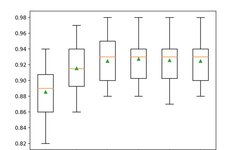
One important hyperparameter for the XGBoost ensemble algorithm is the number of decision trees used in the ensemble. Recall that decision trees are added sequentially to the model to correct and improve the predictions of the existing trees. Thus, more trees are usually better. The number of trees can be set via the n_estimators parameter, which defaults to 100. Below is an example that explores the effect of the number of trees with values ranging from 10 to 5,000.

# explore xgboost number of trees effect on performance
from numpy import mean
from numpy import std
from sklearn.datasets import make_classification
from sklearn.model_selection import cross_val_score
from sklearn.model_selection import RepeatedStratifiedKFold
from xgboost import XGBClassifier
from matplotlib import pyplot

# get the dataset
def get_dataset():
 X, y = make_classification(n_samples=1000, n_features=20, n_informative=15, n_redundant=5, random_state=7)
 return X, y

# get a list of models to evaluate
def get_models():
 models = dict()
 trees = [10, 50, 100, 500, 1000, 5000]
 for n in trees:
  models[str(n)] = XGBClassifier(n_estimators=n)
 return models

# evaluate a give model using cross-validation
def evaluate_model(model):
 cv = RepeatedStratifiedKFold(n_splits=10, n_repeats=3, random_state=1)
 scores = cross_val_score(model, X, y, scoring='accuracy', cv=cv, n_jobs=-1)
 return scores

# define dataset
X, y = get_dataset()
# get the models to evaluate
models = get_models()
# evaluate the models and store results
results, names = list(), list()
for name, model in models.items():
 scores = evaluate_model(model)
 results.append(scores)
 names.append(name)
 print('>%s %.3f (%.3f)' % (name, mean(scores), std(scores)))
# plot model performance for comparison
pyplot.boxplot(results, labels=names, showmeans=True)
pyplot.show()

Running the example will report the mean accuracy for each configured number of decision trees.

In this case, we can see that performance improves for the dataset until about 500 trees, after which performance seems to stabilize or decline.

>10 0.885 (0.029)
>50 0.915 (0.029)
>100 0.925 (0.028)
>500 0.927 (0.028)
>1000 0.926 (0.028)
>5000 0.925 (0.027)

Create a box plot to distribute the accuracy scores for each configuration of the number of trees. We can see the overall trend of increasing model performance with ensemble size.

Extreme Gradient Boosting (XGBoost) Ensemble in Python

Exploring Tree Depth

Another important hyperparameter for gradient boosting is the depth of each tree added to the ensemble. The depth of the trees controls how specialized each tree is to the training dataset: the generality or overfitting of the tree. Ideally, the trees should not be too shallow and general (like AdaBoost) nor too deep and specialized (like bagging). Gradient boosting typically performs well with trees of moderate depth, thus finding a balance between specificity and generality. 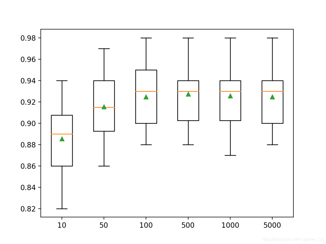The depth of the trees is controlled by the max_depth parameter, which defaults to 6. Below is an example that explores the tree depth from 1 to 10 and its effect on model performance.

# explore xgboost tree depth effect on performance
from numpy import mean
from numpy import std
from sklearn.datasets import make_classification
from sklearn.model_selection import cross_val_score
from sklearn.model_selection import RepeatedStratifiedKFold
from xgboost import XGBClassifier
from matplotlib import pyplot

# get the dataset
def get_dataset():
 X, y = make_classification(n_samples=1000, n_features=20, n_informative=15, n_redundant=5, random_state=7)
 return X, y

# get a list of models to evaluate
def get_models():
 models = dict()
 for i in range(1,11):
  models[str(i)] = XGBClassifier(max_depth=i)
 return models

# evaluate a give model using cross-validation
def evaluate_model(model):
 cv = RepeatedStratifiedKFold(n_splits=10, n_repeats=3, random_state=1)
 scores = cross_val_score(model, X, y, scoring='accuracy', cv=cv, n_jobs=-1)
 return scores

# define dataset
X, y = get_dataset()
# get the models to evaluate
models = get_models()
# evaluate the models and store results
results, names = list(), list()
for name, model in models.items():
 scores = evaluate_model(model)
 results.append(scores)
 names.append(name)
 print('>%s %.3f (%.3f)' % (name, mean(scores), std(scores)))
# plot model performance for comparison
pyplot.boxplot(results, labels=names, showmeans=True)
pyplot.show()

Running the example will report the mean accuracy for each configured tree depth.

In this case, we can see that performance improves with tree depth, peaking around 3 to 8 depth, after which deeper, more specialized trees result in worse performance.

>1 0.849 (0.028)
>2 0.906 (0.032)
>3 0.926 (0.027)
>4 0.930 (0.027)
>5 0.924 (0.031)
>6 0.925 (0.028)
>7 0.926 (0.030)
>8 0.926 (0.029)
>9 0.921 (0.032)
>10 0.923 (0.035)

Create a box plot to distribute the accuracy scores for each configured tree depth. We can see the overall trend of model performance peaking at a certain depth, after which performance begins to stabilize or decline due to overly specialized trees.

Extreme Gradient Boosting (XGBoost) Ensemble in Python

Exploring Learning Rate

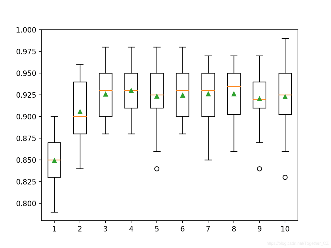
The learning rate controls how much each model contributes to the overall prediction. A lower rate may require more decision trees in the ensemble. The learning rate can be controlled via the eta parameter, which defaults to 0.3. Below is an example that explores the learning rate and compares values between 0.0001 and 1.0.

# explore xgboost learning rate effect on performance
from numpy import mean
from numpy import std
from sklearn.datasets import make_classification
from sklearn.model_selection import cross_val_score
from sklearn.model_selection import RepeatedStratifiedKFold
from xgboost import XGBClassifier
from matplotlib import pyplot

# get the dataset
def get_dataset():
 X, y = make_classification(n_samples=1000, n_features=20, n_informative=15, n_redundant=5, random_state=7)
 return X, y

# get a list of models to evaluate
def get_models():
 models = dict()
 rates = [0.0001, 0.001, 0.01, 0.1, 1.0]
 for r in rates:
  key = '%.4f' % r
  models[key] = XGBClassifier(eta=r)
 return models

# evaluate a give model using cross-validation
def evaluate_model(model):
 cv = RepeatedStratifiedKFold(n_splits=10, n_repeats=3, random_state=1)
 scores = cross_val_score(model, X, y, scoring='accuracy', cv=cv, n_jobs=-1)
 return scores

# define dataset
X, y = get_dataset()
# get the models to evaluate
models = get_models()
# evaluate the models and store results
results, names = list(), list()
for name, model in models.items():
 scores = evaluate_model(model)
 results.append(scores)
 names.append(name)
 print('>%s %.3f (%.3f)' % (name, mean(scores), std(scores)))
# plot model performance for comparison
pyplot.boxplot(results, labels=names, showmeans=True)
pyplot.show()

Running the example will report the mean accuracy for each configured learning rate.

In this case, we can see that a higher learning rate results in better performance for this dataset. We hope that adding more trees to the ensemble with a smaller learning rate will further improve performance.

This highlights the trade-off between the number of trees (training speed) and learning rate, for example, we can fit the model faster with fewer trees and a larger learning rate.

>0.0001 0.804 (0.039)
>0.0010 0.814 (0.037)
>0.0100 0.867 (0.027)
>0.1000 0.923 (0.030)
>1.0000 0.913 (0.030)

Create a box plot to distribute the accuracy scores for each configured learning rate. We can see the overall trend of increasing model performance with increasing learning rate, peaking at 0.1, after which performance declines.

Extreme Gradient Boosting (XGBoost) Ensemble in Python

Exploring Sample Size

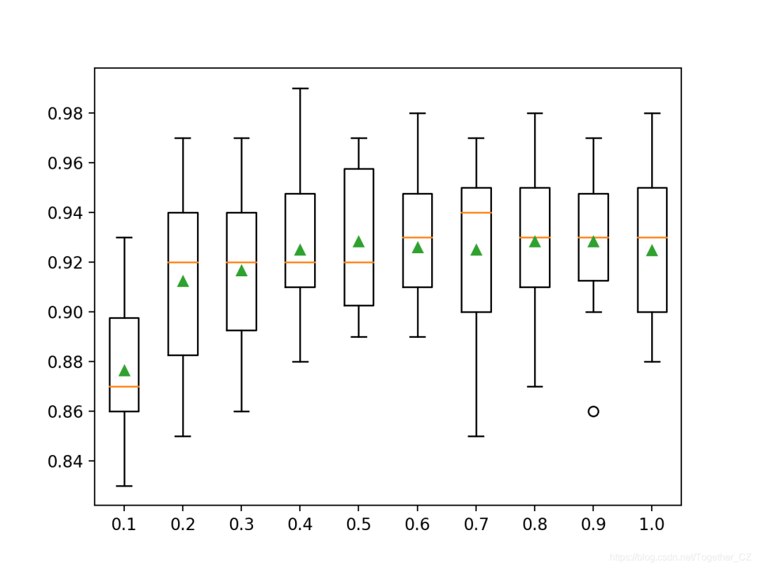
The number of samples used to fit each tree can vary. This means that each tree is fitted to a random subset of the training dataset. Using fewer samples introduces more variance for each tree, although it can improve overall model performance. The number of samples used to fit each tree is specified by the subsample parameter and can be set to a small fraction of the training dataset size. By default, it is set to 1.0 to use the entire training dataset. Below is an example that demonstrates the effect of sample size on model performance, varying the ratio from 10% to 100% in 10% increments.

# explore xgboost subsample ratio effect on performance
from numpy import arange
from numpy import mean
from numpy import std
from sklearn.datasets import make_classification
from sklearn.model_selection import cross_val_score
from sklearn.model_selection import RepeatedStratifiedKFold
from xgboost import XGBClassifier
from matplotlib import pyplot

# get the dataset
def get_dataset():
 X, y = make_classification(n_samples=1000, n_features=20, n_informative=15, n_redundant=5, random_state=7)
 return X, y

# get a list of models to evaluate
def get_models():
 models = dict()
 for i in arange(0.1, 1.1, 0.1):
  key = '%.1f' % i
  models[key] = XGBClassifier(subsample=i)
 return models

# evaluate a give model using cross-validation
def evaluate_model(model):
 cv = RepeatedStratifiedKFold(n_splits=10, n_repeats=3, random_state=1)
 scores = cross_val_score(model, X, y, scoring='accuracy', cv=cv, n_jobs=-1)
 return scores

# define dataset
X, y = get_dataset()
# get the models to evaluate
models = get_models()
# evaluate the models and store results
results, names = list(), list()
for name, model in models.items():
 scores = evaluate_model(model)
 results.append(scores)
 names.append(name)
 print('>%s %.3f (%.3f)' % (name, mean(scores), std(scores)))
# plot model performance for comparison
pyplot.boxplot(results, labels=names, showmeans=True)
pyplot.show()

Running the example will report the mean accuracy for each configured sample size.

In this case, we can see that average performance may be best for sample sizes covering most datasets (around 80% or higher).

>0.1 0.876 (0.027)
>0.2 0.912 (0.033)
>0.3 0.917 (0.032)
>0.4 0.925 (0.026)
>0.5 0.928 (0.027)
>0.6 0.926 (0.024)
>0.7 0.925 (0.031)
>0.8 0.928 (0.028)
>0.9 0.928 (0.025)
>1.0 0.925 (0.028)

Create a box plot to distribute the accuracy scores for each configured sample rate. We can see the overall trend of increasing model performance, possibly peaking around 80% coverage and then leveling off.

Extreme Gradient Boosting (XGBoost) Ensemble in Python

Exploring Feature Count

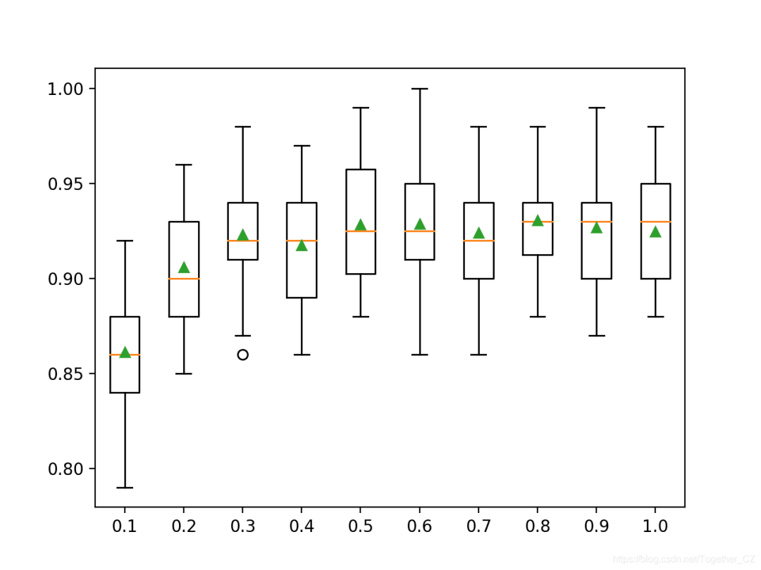
The number of features used to fit each decision tree can vary. Similar to changing the sample size, changing the number of features can also introduce additional variance in the model, although it may require increasing the number of trees to improve performance. The number of features used by each tree is drawn as a random sample and is specified by the colsample_bytree parameter and defaults to using all features in the training dataset, such as 100% or a value of 1.0. You can also sample columns for each split, which is controlled by the colsample_bylevel parameter, but we will not discuss this hyperparameter here. Below is an example that explores the effect of feature count on model performance, varying the ratio from 10% to 100% in 10% increments.

# explore xgboost column ratio per tree effect on performance
from numpy import arange
from numpy import mean
from numpy import std
from sklearn.datasets import make_classification
from sklearn.model_selection import cross_val_score
from sklearn.model_selection import RepeatedStratifiedKFold
from xgboost import XGBClassifier
from matplotlib import pyplot

# get the dataset
def get_dataset():
 X, y = make_classification(n_samples=1000, n_features=20, n_informative=15, n_redundant=5, random_state=7)
 return X, y

# get a list of models to evaluate
def get_models():
 models = dict()
 for i in arange(0.1, 1.1, 0.1):
  key = '%.1f' % i
  models[key] = XGBClassifier(colsample_bytree=i)
 return models

# evaluate a give model using cross-validation
def evaluate_model(model):
 cv = RepeatedStratifiedKFold(n_splits=10, n_repeats=3, random_state=1)
 scores = cross_val_score(model, X, y, scoring='accuracy', cv=cv, n_jobs=-1)
 return scores

# define dataset
X, y = get_dataset()
# get the models to evaluate
models = get_models()
# evaluate the models and store results
results, names = list(), list()
for name, model in models.items():
 scores = evaluate_model(model)
 results.append(scores)
 names.append(name)
 print('>%s %.3f (%.3f)' % (name, mean(scores), std(scores)))
# plot model performance for comparison
pyplot.boxplot(results, labels=names, showmeans=True)
pyplot.show()

Running the example will report the mean accuracy for each configured column ratio.

In this case, we can see that average performance improves to around half (50%) of the feature count, and then levels off afterward. Surprisingly, removing half of the input variables has little effect.

>0.1 0.861 (0.033)
>0.2 0.906 (0.027)
>0.3 0.923 (0.029)
>0.4 0.917 (0.029)
>0.5 0.928 (0.030)
>0.6 0.929 (0.031)
>0.7 0.924 (0.027)
>0.8 0.931 (0.025)
>0.9 0.927 (0.033)
>1.0 0.925 (0.028)

Create a box plot to distribute the accuracy scores for each configured column ratio. We can see the overall trend of improving model performance possibly peaking at around 60% feature count and then leveling off.

Extreme Gradient Boosting (XGBoost) Ensemble in Python

Author: Yishui Hancheng, CSDN Blog Expert, personal research direction: Machine Learning, Deep Learning, NLP, CV

Blog: http://yishuihancheng.blog.csdn.net

Appreciate the Author

Leave a Comment Cancel reply