

Source: I learned at Xuecheng

This article is about 3400 words and is recommended to read in 5 minutes.
It evaluates the performance of models from the perspectives of speed and accuracy.
Boosting algorithms are a class of machine learning algorithms that build a strong classifier by iteratively training a series of weak classifiers (usually decision trees). In each round of iteration, the new classifier is designed to correct the errors of the previous round’s classifier, thereby gradually improving overall classification performance.
Despite the rise and popularity of neural networks, boosting algorithms remain quite practical. They still perform well under conditions of limited training data, short training times, and a lack of expertise in parameter tuning.
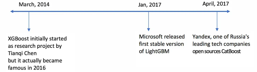
Boosting algorithms include AdaBoost, CatBoost, LightGBM, XGBoost, etc.
This article will focus on CatBoost, LightGBM, and XGBoost. It will include:
– Structural differences;
– How each algorithm handles categorical variables;
– Understanding parameters;
– Practical applications on datasets;
– Performance of each algorithm.
Article from: https://towardsdatascience.com/catboost-vs-light-gbm-vs-xgboost-5f93620723db
To suit Chinese reading habits and enhance immersion, the original text has been translated and edited.
Hunter Phillips | Author
Robert | Editor
Since XGBoost (often referred to as the GBM Killer) has been around in the machine learning field for a long time and there are many articles dedicated to it, this article will focus more on CatBoost and LGBM.
1. Structural Differences Between LightGBM and XGBoost
LightGBM uses a novel Gradient-based One-Side Sampling (GOSS) technique to filter data instances when searching for split values, while XGBoost uses a pre-sorted algorithm and a histogram-based algorithm to calculate the best splits.
The above instances refer to observations/samples.
First, let’s understand how XGBoost’s pre-sorted splitting works:
-
For each node, enumerate all features; -
For each feature, sort instances by feature value; -
Use a linear scan to determine the best split on that feature based on information gain; -
Select the best split solution among all features.
In simple terms, the histogram-based algorithm divides all data points of the feature into discrete bins and uses these bins to find the split value of the histogram. Although it is more efficient in training speed than the pre-sorted algorithm, which requires enumerating all possible split points on pre-sorted feature values, it still lags behind GOSS in speed.
So, what makes the GOSS method efficient?
In AdaBoost, sample weights can serve as a good indicator of sample importance. However, in Gradient Boosting Decision Trees (GBDT), there are no native sample weights, so the sampling method proposed by AdaBoost cannot be applied directly. This introduces a gradient-based sampling method.
The gradient represents the slope of the loss function’s tangent, so in a sense, if a data point has a large gradient, it is important for finding the best split point because it has a higher error.
GOSS retains all instances with large gradients and randomly samples instances with small gradients. For example, suppose I have 500,000 rows of data, of which 10,000 rows have large gradients. Therefore, my algorithm will select (10k rows with large gradients + x% randomly selected from the remaining 490k rows). Assuming x is 10%, the total number of selected rows is 59k, and the split value is found based on these rows.
The basic assumption here is that training instances with smaller gradients have smaller training errors and have already been well trained. To maintain the same data distribution, GOSS introduces a constant multiplier for data instances with smaller gradients when calculating information gain. Thus, GOSS achieves a good balance between reducing the number of data instances and maintaining the accuracy of learning decision trees.
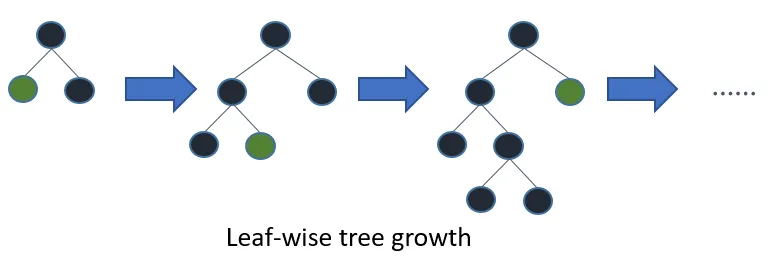
LGBM further grows on leaves with greater gradients/errors.
2. How Each Model Handles Categorical Variables?
2.1 CatBoost
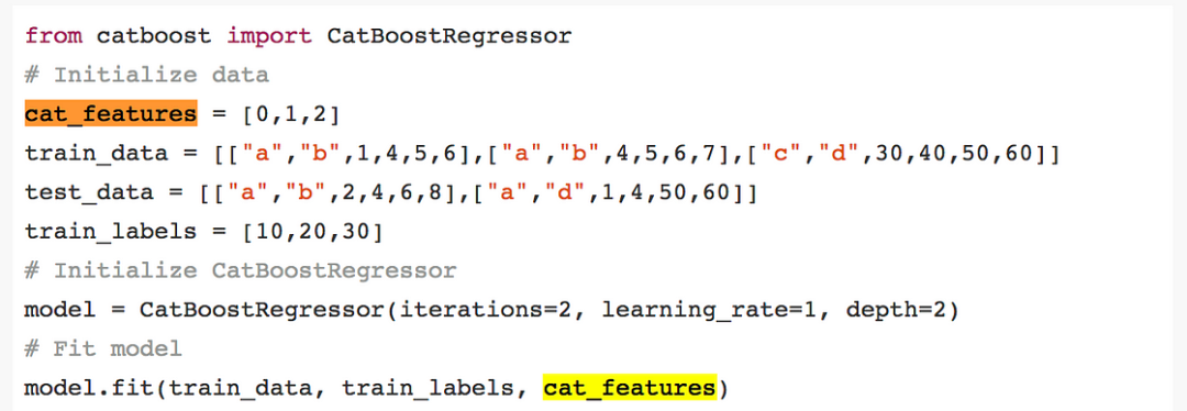
CatBoost has the flexibility to provide the indices of categorical columns so that one-hot encoding can be used, utilizing the one_hot_max_size parameter (one-hot encoding is applied to all features with a number of different values less than or equal to the given parameter value).
If nothing is passed in the cat_features parameter, CatBoost will treat all columns as numerical variables.
Note: If a column containing string values is not provided in cat_features, CatBoost will throw an error. Additionally, columns that default to int type will be treated as numerical by default, and if they are to be treated as categorical variables, they must be specified in cat_features.
For the remaining categorical columns where the number of unique categories is greater than one_hot_max_size, CatBoost uses an efficient encoding method similar to mean encoding that reduces overfitting. The process is as follows:
-
Randomly shuffle the input observation set in random order to generate multiple random permutations; -
Convert label values from float or category to integer; -
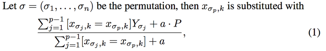
Use the following formula to convert all categorical feature values to numerical:
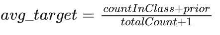
Where countInClass represents the occurrence count of the current categorical feature value in objects where the label value equals “1”, prior is the initial value of the numerator determined by the starting parameters, and totalCount is the total number of objects prior to the current object that match the current categorical feature value.
Mathematically, it can be represented by the following equation:
2.2 LightGBM
Similar to CatBoost, LightGBM can also handle categorical features by inputting feature names. It does not convert to one-hot encoding and is much faster than one-hot encoding. LGBM uses a special algorithm to find split values for categorical features.
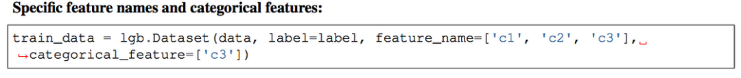
Note: Before building the LGBM dataset, you should convert categorical features to integer type. Even if string values are passed through the categorical_feature parameter, it does not accept string values.
2.3 XGBoost
Unlike CatBoost or LGBM, XGBoost cannot handle categorical features natively; it only accepts numerical data similar to random forests. Therefore, various encodings such as label encoding, mean encoding, or one-hot encoding need to be performed before providing categorical data to XGBoost.
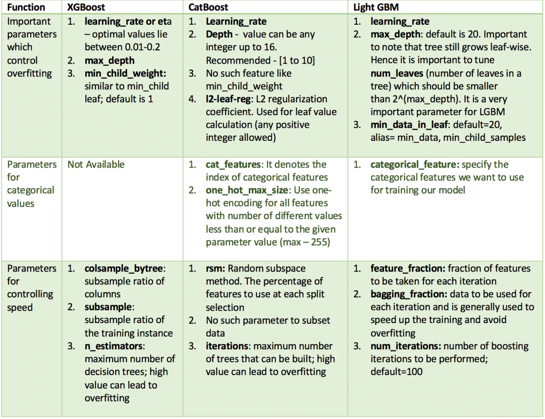
3. Understanding Parameters
All these models have many parameters to tune, but we will only discuss the important ones. Below is a list of these parameters based on their functionality and corresponding parameters in different models.
4. Implementation on Datasets
I used the Kaggle dataset of flight delays from 2015 because it contains both categorical and numerical features. With about 5 million rows of data, this dataset is good for evaluating the performance of each type of boosting model in terms of speed and accuracy. I will use a 10% subset of this data, about 500,000 rows.
Here are the features used for modeling:
-
MONTH, DAY, DAY_OF_WEEK: data type int -
AIRLINE and FLIGHT_NUMBER: data type int -
ORIGIN_AIRPORT and DESTINATION_AIRPORT: data type string -
DEPARTURE_TIME: data type float -
ARRIVAL_DELAY: this will be the target variable and converted to a boolean variable representing delays over 10 minutes -
DISTANCE and AIR_TIME: data type float
import pandas as pd, numpy as np, time
from sklearn.model_selection import train_test_split
data = pd.read_csv("./data/flights.csv")
data = data.sample(frac = 0.1, random_state=10)
data = data[["MONTH","DAY","DAY_OF_WEEK","AIRLINE","FLIGHT_NUMBER","DESTINATION_AIRPORT", "ORIGIN_AIRPORT","AIR_TIME", "DEPARTURE_TIME","DISTANCE","ARRIVAL_DELAY"]]
data.dropna(inplace=True)
data["ARRIVAL_DELAY"] = (data["ARRIVAL_DELAY"]>10)*1
cols = ["AIRLINE","FLIGHT_NUMBER","DESTINATION_AIRPORT","ORIGIN_AIRPORT"]
for item in cols:    data[item] = data[item].astype("category").cat.codes + 1
train, test, y_train, y_test = train_test_split(data.drop(["ARRIVAL_DELAY"], axis=1), data["ARRIVAL_DELAY"],random_state=10, test_size=0.25)

4.1 XGBoost
import xgboost as xgb
from sklearn import metrics
from sklearn.model_selection import GridSearchCV
def auc(m, train, test):     return (metrics.roc_auc_score(y_train,m.predict_proba(train)[:,1]),                            metrics.roc_auc_score(y_test,m.predict_proba(test)[:,1]))
# Parameter Tuning
model = xgb.XGBClassifier()
param_dist = {"max_depth": [10,30,50],              "min_child_weight" : [1,3,6],              "n_estimators": [200],              "learning_rate": [0.05, 0.1,0.16],}
grid_search = GridSearchCV(model, param_grid=param_dist, cv = 3,                                    verbose=10, n_jobs=-1)
grid_search.fit(train, y_train)
grid_search.best_estimator_
model = xgb.XGBClassifier(max_depth=50, min_child_weight=1,  n_estimators=200,
                          n_jobs=-1 , verbose=1,learning_rate=0.16)
model.fit(train,y_train)
auc(model, train, test)

4.2 LightGBM
import lightgbm as lgb
from sklearn import metrics
def auc2(m, train, test):     return (metrics.roc_auc_score(y_train,m.predict(train)),                            metrics.roc_auc_score(y_test,m.predict(test)))
lg = lgb.LGBMClassifier(verbose=0)
param_dist = {"max_depth": [25,50, 75],              "learning_rate" : [0.01,0.05,0.1],              "num_leaves": [300,900,1200],              "n_estimators": [200]             }
grid_search = GridSearchCV(lg, n_jobs=-1, param_grid=param_dist, cv = 3, scoring="roc_auc", verbose=5)
grid_search.fit(train,y_train)
grid_search.best_estimator_
d_train = lgb.Dataset(train, label=y_train)
params = {"max_depth": 50, "learning_rate" : 0.1, "num_leaves": 900,  "n_estimators": 300}
# Without Categorical Features
model2 = lgb.train(params, d_train)
auc2(model2, train, test)
# With Categorical Features
cate_features_name = ["MONTH","DAY","DAY_OF_WEEK","AIRLINE","DESTINATION_AIRPORT", "ORIGIN_AIRPORT"]
model2 = lgb.train(params, d_train, categorical_feature = cate_features_name)
auc2(model2, train, test)
4.3 CatBoost
When tuning parameters for CatBoost, it is difficult to pass the indices of categorical features. Therefore, I tuned parameters without passing categorical features and evaluated two models – one using categorical features and the other not. I adjusted one_hot_max_size separately as it does not affect other parameters.
import catboost as cb
cat_features_index = [0,1,2,3,4,5,6]
def auc(m, train, test):     return (metrics.roc_auc_score(y_train,m.predict_proba(train)[:,1]),                            metrics.roc_auc_score(y_test,m.predict_proba(test)[:,1]))
params = {'depth': [4, 7, 10],          'learning_rate' : [0.03, 0.1, 0.15],         'l2_leaf_reg': [1,4,9],         'iterations': [300]}cb = cb.CatBoostClassifier()
cb_model = GridSearchCV(cb, params, scoring="roc_auc", cv = 3)
cb_model.fit(train, y_train)
# With Categorical features
clf = cb.CatBoostClassifier(eval_metric="AUC", depth=10, iterations= 500, l2_leaf_reg= 9, learning_rate= 0.15)
clf.fit(train,y_train)
auc(clf, train, test)
# With Categorical features
clf = cb.CatBoostClassifier(eval_metric="AUC",one_hot_max_size=31,
                            depth=10, iterations= 500, l2_leaf_reg= 9, learning_rate= 0.15)
clf.fit(train,y_train, cat_features= cat_features_index)
auc(clf, train, test)
5. Conclusion
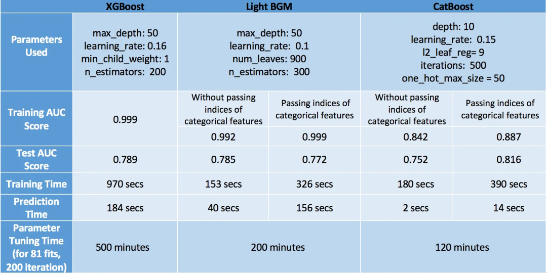
When evaluating models, we should consider model performance from both speed and accuracy perspectives.
With this in mind, CatBoost is the winner, achieving the highest accuracy on the test set (0.816), minimal overfitting (accuracy on training and test sets are close), and the shortest prediction and tuning times. However, this is only because we considered categorical variables and tuned one_hot_max_size correctly. If we do not leverage these features of CatBoost, its accuracy is only 0.752, performing the worst. Therefore, we conclude that CatBoost performs well only when categorical variables are present in the data, and we tune them correctly.
Our next best-performing model is XGBoost. Even ignoring the fact that we had categorical variables in the data and converted them to numerical variables for XGBoost, its accuracy is still quite close to that of CatBoost. However, the only issue with XGBoost is its slow speed. Tuning its parameters is really frustrating, especially using GridSearchCV (running GridSearchCV took me 6 hours, a very bad idea!). A better approach is to tune parameters individually rather than using GridSearchCV. Read this blog post to learn how to tune parameters cleverly.
Finally, LightGBM ranks last. One point to note here is that it performs poorly in terms of speed and accuracy when using cat_features. I believe its poor performance is due to its use of a modified mean encoding for categorical data, leading to overfitting (very high training accuracy – 0.999, in contrast to low test accuracy). However, if it is used normally like XGBoost, it can achieve similar (or even higher) accuracy at a much faster speed (LGBM – 0.785, XGBoost – 0.789).
Finally, I must say that these observations apply to this specific dataset and may or may not hold for other datasets. However, in general, a real situation is that XGBoost is slower than the other two algorithms.
Editor: Huang Jiyan