

Selecting the right LLM inference stack means choosing the right model for your task and running appropriate inference code on suitable hardware. This article introduces popular LLM inference stacks and setups, detailing their cost composition for inference; it also discusses current open-source models and how to make the most of them, while addressing features that are still missing in the current open-source service stack and new functionalities that future models will unlock.
Author | Timothée Lacroix
Compiled by OneFlow
Translation | Wan Zilin, Yang Ting
Much of the content of this talk is based on information I found online or discoveries made while experimenting with the first version of the LLaMA model. I believe that Mistral is now more focused on inference costs rather than training costs. Therefore, I will share the composition of inference costs, throughput, latency, and their influencing factors.
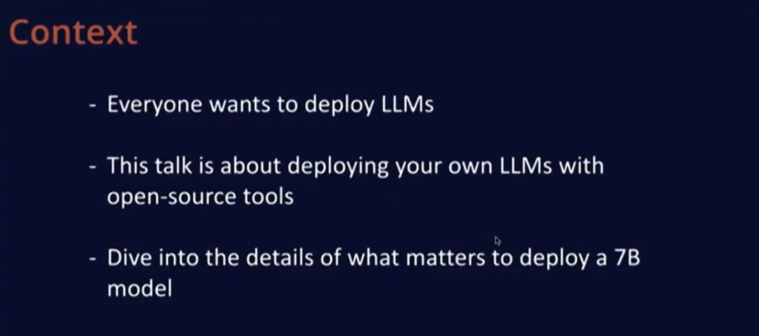
Many people want to deploy large language models, and I will share how to deploy your own language model using open-source tools. Of course, you can also use some excellent public APIs, but I am more interested in open-source tools, so I will delve into the important details of deploying a 7 billion parameter model next. Much of what I will share also applies to larger models, but that requires more GPUs.
1
Metrics Affecting Inference
We will first discuss what important metrics exist and the factors that influence these metrics, including both hardware and software aspects. Next, I will introduce some tips that can improve performance; as far as I know, some of these tips have not yet been widely implemented. I have tried running a series of models on various hardware and attempted to obtain performance curves; I believe instances are very important, so I will draw conclusions based on this data.
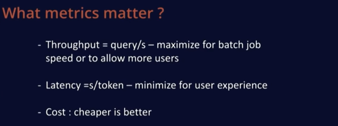
First, what metrics should we focus on? The first is throughput, expressed as queries per second (Query/second); we want to maximize this metric in batch jobs or allow more users to use our service. The second is latency, expressed as seconds per token (seconds/token), which is the time required to output the next token; this determines the speed and responsiveness of your application. In ChatGPT, this speed is quite fast. Smaller models can achieve quick responses more easily, so we want to minimize this value to enhance user experience. A good threshold is 250 words per minute, which I believe is the average reading speed of humans; as long as your latency is below this value, users will not feel bored. The third is cost; undoubtedly, the lower this value, the better.
2
Factors Affecting Inference Metrics
Now I will delve into the factors affecting these metrics. I will only discuss autoregressive decoding, which determines the next batch of tokens based on batches of tokens through a neural network; this part does not include processing the first part of the query. Prompt processing is sometimes referred to as the prefill phase, where we input a large number of tokens into the neural network at once; this part of processing is usually well optimized, and the challenges are relatively low.
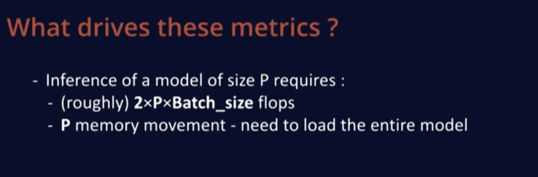
With this in mind, we are interested in the inference of a model of size P. It can be assumed that P is 7B, and to perform one step of inference, approximately 2xPxBatch_size FLOPs (floating point operations) are required. When performing these floating-point operations, we need to load the entire model into the GPU that actually runs the calculations, and the entire model needs to be loaded at once, which roughly requires a memory movement amount equal to the number of parameters in the model.
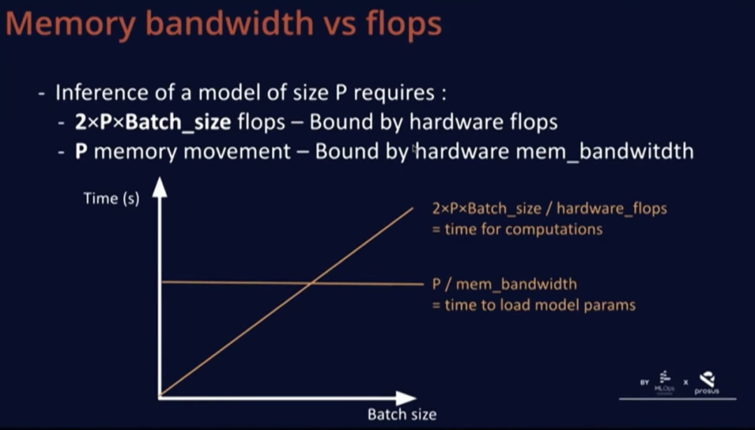
These two quantities are interesting in that the first quantity is limited by the hardware’s floating-point computing capability, that is, the number of floating-point operations the GPU can achieve, and it is linearly related to the batch size, presenting a growth trend in the above graph. Unless the batch size is particularly large, the memory movement amount does not change with the batch size. But as I said, this situation has been optimized to a considerable extent, so we are not too concerned about memory movement. We also have a constant, which is the model size divided by memory bandwidth, which is the shortest time required to load the entire model at once; this operation needs to be performed again each time.
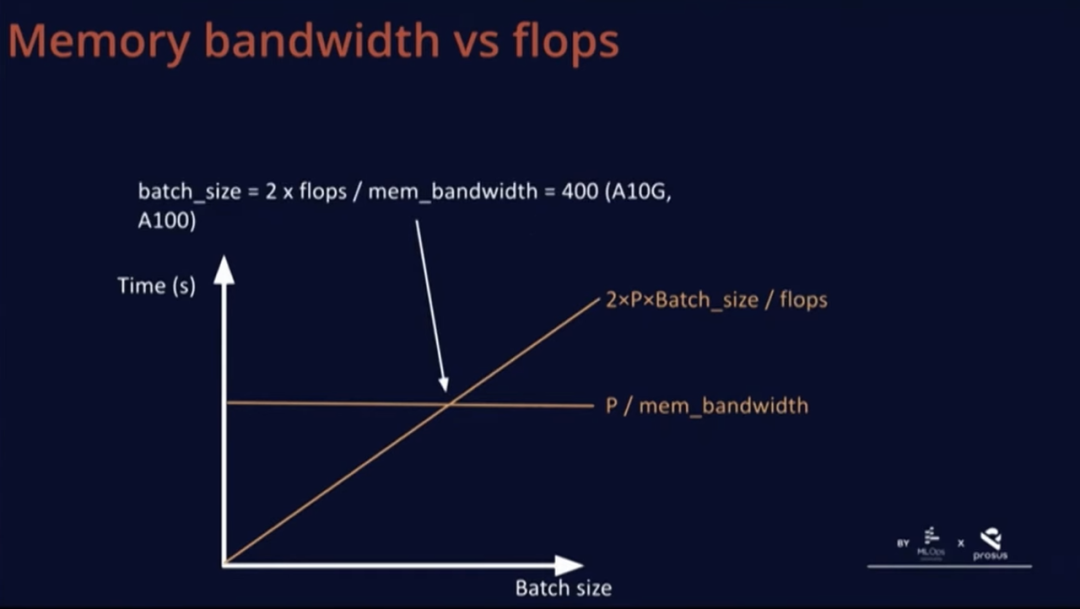
There is also a quantity related to batch size that intersects at an interesting point. This point does not depend on any factors beyond hardware. For example, on A10G and A100, the total number of floating-point operations that the hardware can achieve divided by memory bandwidth is 400.
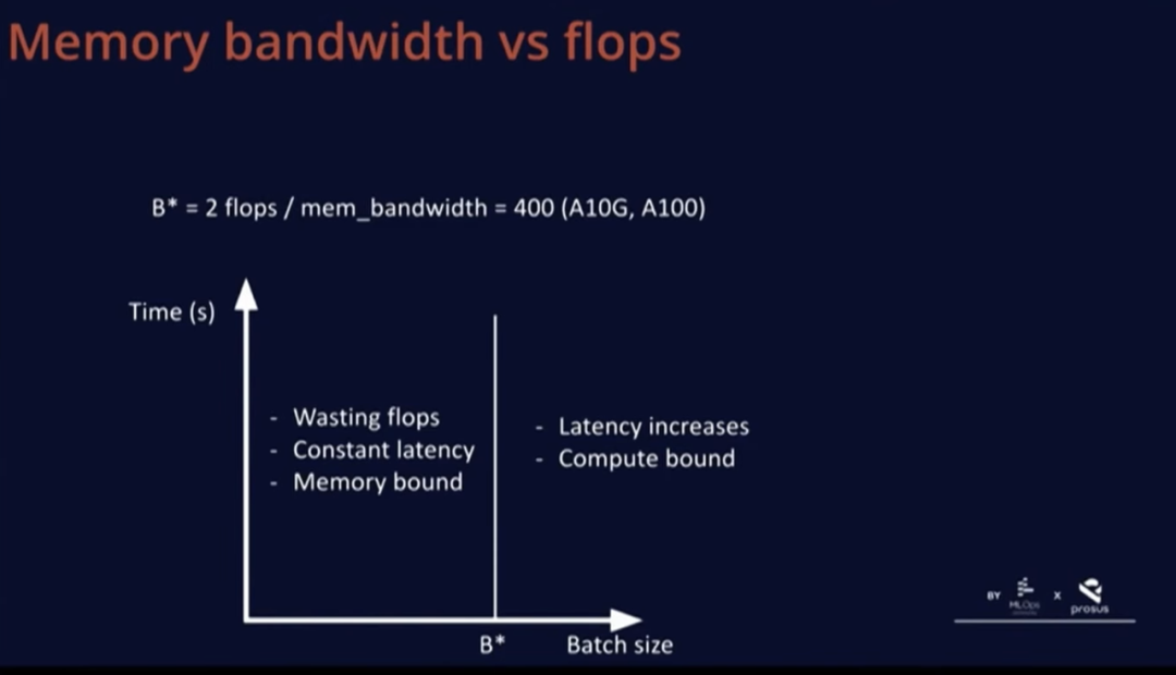
B* is a very interesting batch size because below this batch size, we are essentially wasting FLOPs as computation is limited by memory; we are waiting for the GPU to load data while the computation speed is too fast, resulting in a constant latency in some parts of the graph. If we exceed this threshold B*, latency will start to increase, becoming computation-limited.
Therefore, the true advantage of B* is that the latency range at this batch size is optimal, resulting in the best user experience without wasting any FLOPs.
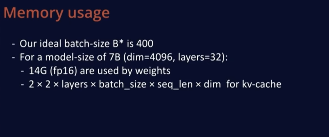
In any case, our ideal batch size B* is 400, which seems quite large, so let’s calculate some metrics for models like LLaMA. The LLaMA model has 4K dimensions and 32 layers, making the model size easy to calculate; in FP16, each model weight occupies two bytes, so it only requires 2×7=14GB of memory.
Then, we use a KV cache to store computation results so that when we re-encode a new token, we do not have to recompute from scratch. The KV cache size is 2, including K cache and V cache, and using FP16 format, each is multiplied by 2, and there must be a KV cache for each layer, which must save data for each element in the batch, with each position in the sequence representing a token, then multiplied by the dimension.
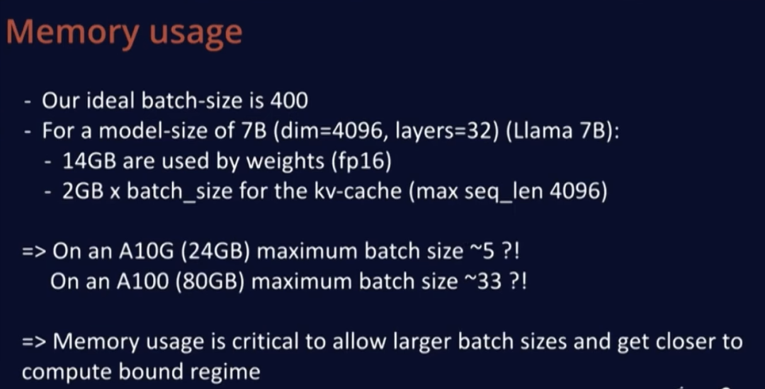
Substituting actual values into this formula reveals that each batch element requires about 2G of memory to support a maximum length of 4K; therefore, on A10 (24GB memory), our maximum batch size is about 5, while on the larger A100 (80GB memory), the maximum batch size is only around 33, which is still far below the ideal value of 400.
Therefore, for all practical use cases, using a 7 billion parameter model for inference, the decoding process will be severely limited by memory bandwidth. This also proves a point that Mistral has been very cautious about from the beginning: the size of the memory occupied by the model and KV cache indeed affects the maximum allowable batch size, which directly determines the efficiency.
3
Practical Tips
Now I will delve into some existing but personally favored tips. Some of these have already been used by Mistral, while others have not yet been applied in Mistral, and some pertain more to software deployment.
Grouped Query Attention
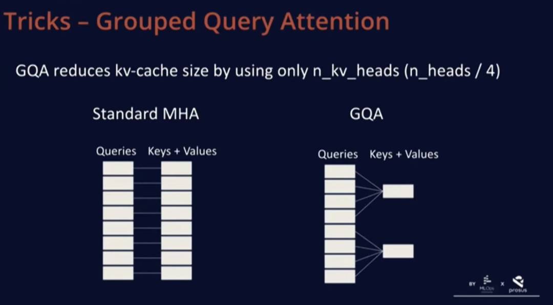
The first tip is grouped query attention. Grouped query attention reduces the KV cache by using fewer keys and values for each query. This has been used in LLaMA 2 but only for larger model sizes, not for the 7 billion parameter model. In standard multi-head attention, there are as many queries as there are keys and values. In grouped query attention, a pair of keys and values is associated with a group of queries. In Mistral, each key and value uses four queries, so the amount of floating-point operations to be performed remains unchanged, but the memory overhead is only a quarter of the original. This is a simple trick that does not significantly harm performance, and this approach is quite good.
Quantization
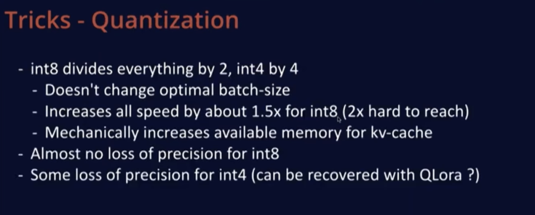
The second tip is quantization, which we have not specifically studied, but especially after the release of LLaMA, this technology has developed very rapidly. Many excellent off-the-shelf solutions are used by many in the open-source community, providing int8 or int4 versions of the model. Using int8 halves the model size, while using int4 reduces it to a quarter.
This does not change the optimal batch size, as this ratio only depends on hardware and is not affected by other factors. In terms of computation speed, the speed after quantization is twice that of the original, but we find it difficult to achieve this speed for Mistral model sizes and others; a 1.5 times speed is more reasonable when measured in pure floating-point operations. Using int8 also mechanically increases the available memory for the KV cache.
Therefore, if you are in a memory-constrained state, everything will operate twice as fast, which is quite nice. Another benefit is that int8 has almost no or very little precision loss, while there will be some performance loss with int4, but this seems to be recoverable through QLoRA, or if you only care about specific use cases, I think this can work normally, and the serving cost will be much lower.
Paged Attention
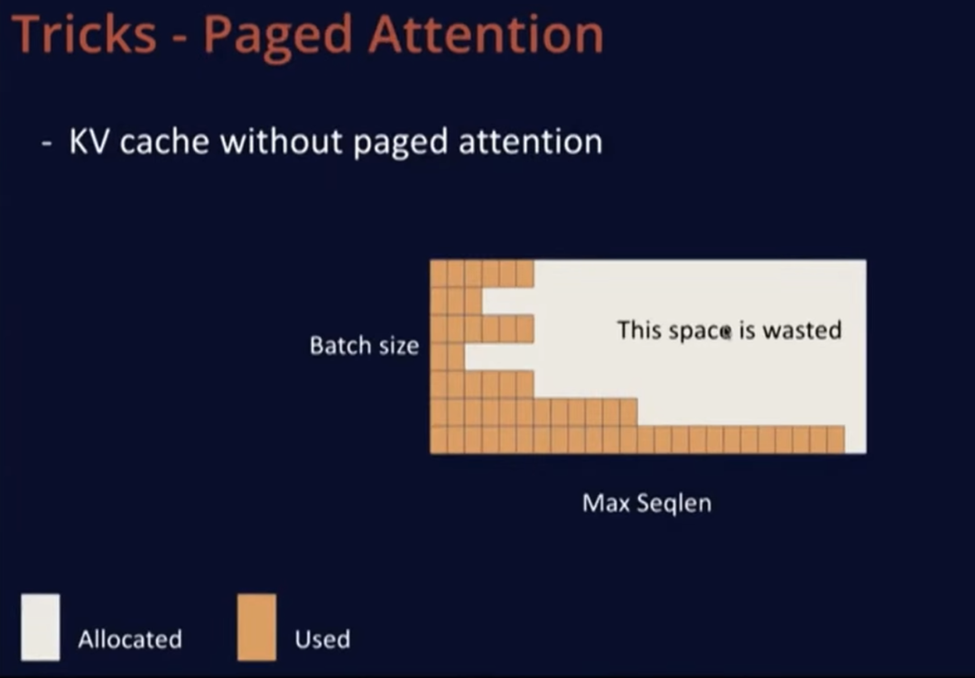
The third tip is paged attention, proposed by vLLM experts from Berkeley. Without paged attention, the KV cache is rectangular and requires allocation of a large rectangular memory, where one dimension is the batch size, which is the maximum number of sequences the model can process at once, and the other dimension is the maximum sequence length allowed for users. When a new sequence comes in, an entire row of memory is allocated for this user, but this is not ideal, as likely only 10% of users will use the entire row of memory, while most users may only initiate short requests. Therefore, this ultimately wastes a lot of valuable space in hardware memory.
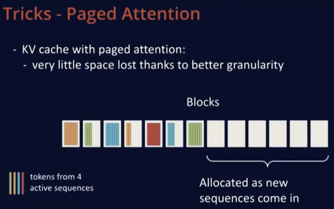
The role of paged attention is to allocate blocks in GPU memory. First, load the model to understand the remaining space size, and then fill the remaining part with memory blocks. These blocks can accommodate up to 16 to 32 tokens, and when a new sequence arrives, the required memory block can be allocated for the prompt and then gradually expanded as needed.
In the above diagram, you can see that the sequences are not necessarily allocated in continuous memory blocks; for example, orange, blue, or green are not in continuous blocks, which is not important. This method allows for finer control of memory allocation, so in the diagram, the completely free part on the right can be used for new incoming sequences, and once the sequence decoding is complete, the used blocks can be released very efficiently. The proposer of paged attention claims that it can increase throughput by about 20 times compared to standard implementation methods, which does not seem so unattainable.
Sliding Window Attention
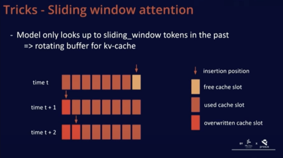
We added a technique in Mistral called sliding window attention. With this technique, we can train the model to use only the past K tokens in the cache. The benefit of this is that we can use a fixed cache size.
As is well known, once a sequence exceeds the number of tokens in the sliding window, we can cyclically overwrite in the cache, starting over without affecting the model’s performance.
Furthermore, through this technique, we can use a longer context length than the sliding window. We have briefly described this in blog posts or on GitHub.
A good implementation of this technique is to view the KV cache as a circular buffer. At time t in the above image, we insert at the last position of the cache; at time t+1, since the sequence exceeds the sliding window, only an overwrite operation is performed. This implementation is very simple because the positions in the cache are not important; all position-related information is encoded through position embeddings. In summary, this method combines ease of implementation and effectiveness.
Continuous Batching
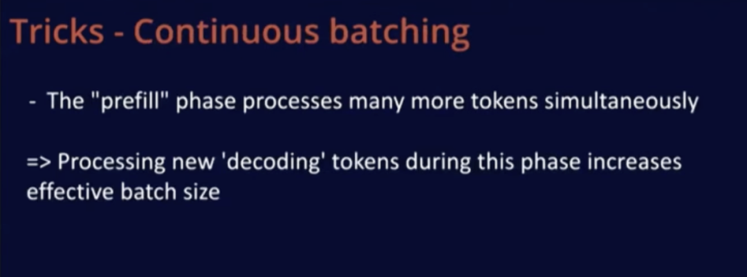
Another tip is continuous batching. As I mentioned earlier, the number of tokens processed simultaneously during the prefill phase is much greater than during the decoding phase. Therefore, we can try to batch these tokens together with the decoding tokens. I have noticed the same issue in both vLLM and TGI, where they have not attempted to chunk the prefill phase. If a user sends a prompt containing 4K tokens to the model, this will increase latency for all users because we need to spend a lot of time processing these tokens at once.
This is actually a waste because at this point, the model is no longer in the optimal state to achieve low latency while fully utilizing computational resources. Therefore, I recommend chunking the prefill in these software solutions, so we only process K tokens at a time. This method allows for finer resource allocation and better batching of decoding and prefill.
Code
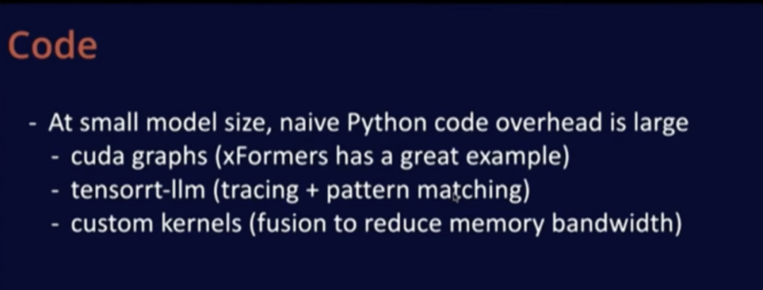
The final technique is code. When dealing with models of this scale, code performance is very important. Typically, we observe that Python code incurs a lot of overhead. Although I have not analyzed the performance of vLLM and TGI in detail, they run Python code, which generally incurs some extra overhead at this scale. We can take some approaches to mitigate this issue without affecting most of the advantages of Python.
The xFormers library is a good example that uses CUDA graphs to achieve zero overhead. NVIDIA’s TensorRT can automatically improve performance by tracking inference and utilizing pattern matching. Additionally, we can use custom kernels (like fusion) to reduce memory bandwidth, thus avoiding moving data back and forth in memory. When data is loaded, we can perform operations like activation, and we can often find optimization tricks for activation functions and easily insert them into the code.
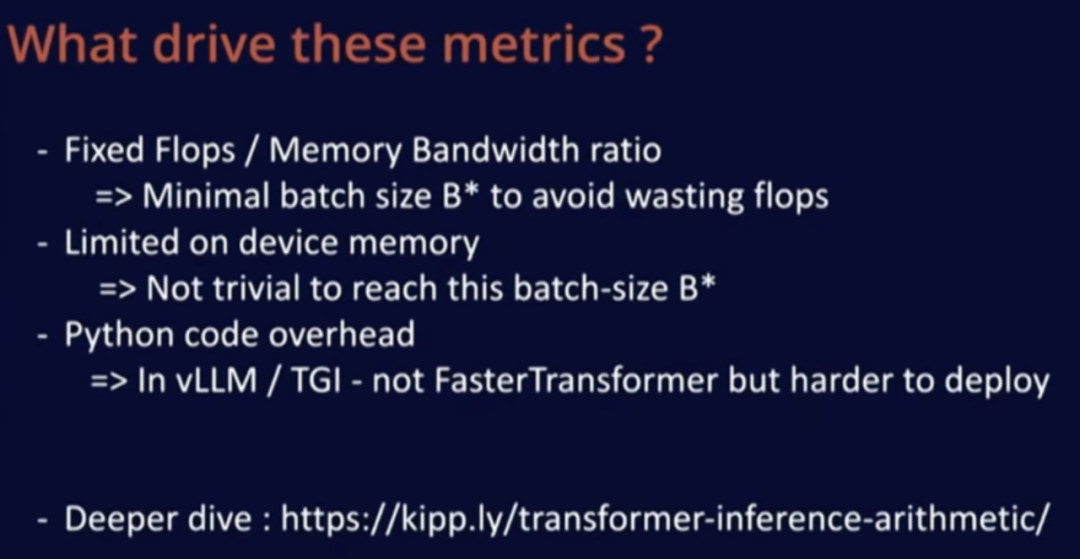
In summary, the factors driving these performance metrics are primarily the ratio of fixed floating-point operations to memory bandwidth in hardware. This gives the minimum batch size B* to fully utilize hardware resources and avoid wasting unnecessary floating-point operations. This size is mainly determined by hardware and is not significantly affected by the model, unless you use a non-traditional architecture other than Transformers. Due to limited device memory, achieving the optimal batch size is not easy.
I checked two open-source libraries for deploying models, which still run Python code; at this scale, the model incurs a lot of extra overhead. I also studied the Faster Transformer project, which has no extra overhead but is more challenging to deploy. The above information mainly comes from the blog post “Inference Calculation of Large Language Models“.
3
Throughput, Latency, and Cost Under Different Configurations
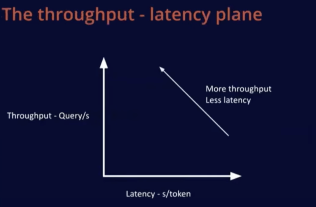
Now let’s talk about the throughput-latency plane graph, which is usually how I judge these metrics. In this plane, the x-axis represents latency, and the y-axis represents throughput; we mainly focus on the upper and left sides, that is, better throughput and lower latency.
Purchasing better hardware will change this throughput-latency performance curve. For fixed hardware, the lower left area is the fixed latency, that is, the memory-constrained area. As the batch size increases, the system transitions from the memory-constrained area to the compute-constrained area. If you purchase more advanced hardware, the cost will be higher, but all curves on the throughput-latency graph will shift overall to the upper left.
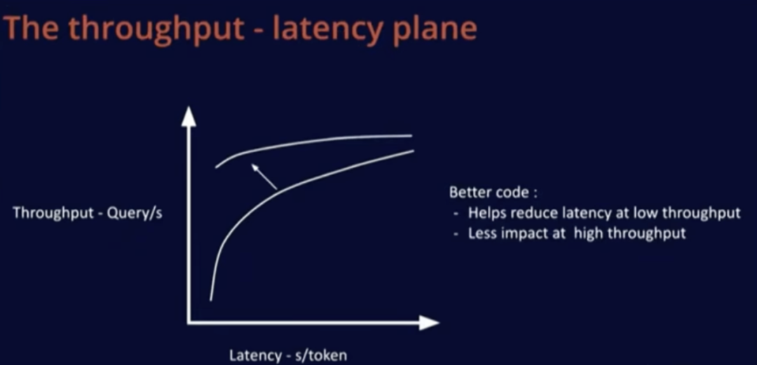
Improving code or adopting better models will have a significant impact in the low-latency area, increasing throughput, which has a smaller effect on large batch sizes since optimization is relatively easy at that point.
Below are some performance test results and disclaimers; this test was completed in a short time because it is easy to configure tools like Mistral and LLaMA, and I ran the vLLM benchmark script. I am not sure if these results are the best I can achieve, but at least the overall direction is correct; below are the Matplotlib graphs I copied and pasted for reference.
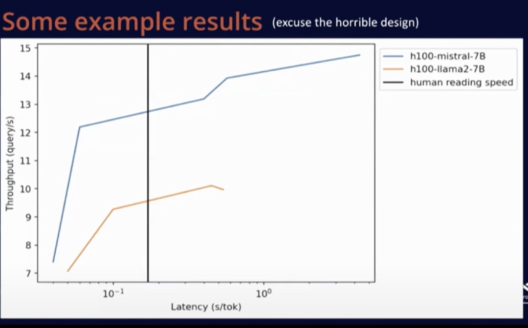
The above graph compares the performance of Mistral and LLaMA. The black line indicates human reading speed.
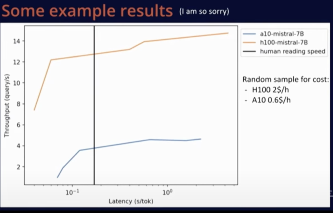
The above graph compares A10 and H100 hardware within the same model. It can be seen that although the H100 is more expensive, replacing hardware is a wiser choice due to its superior performance rather than continuing to use older hardware.
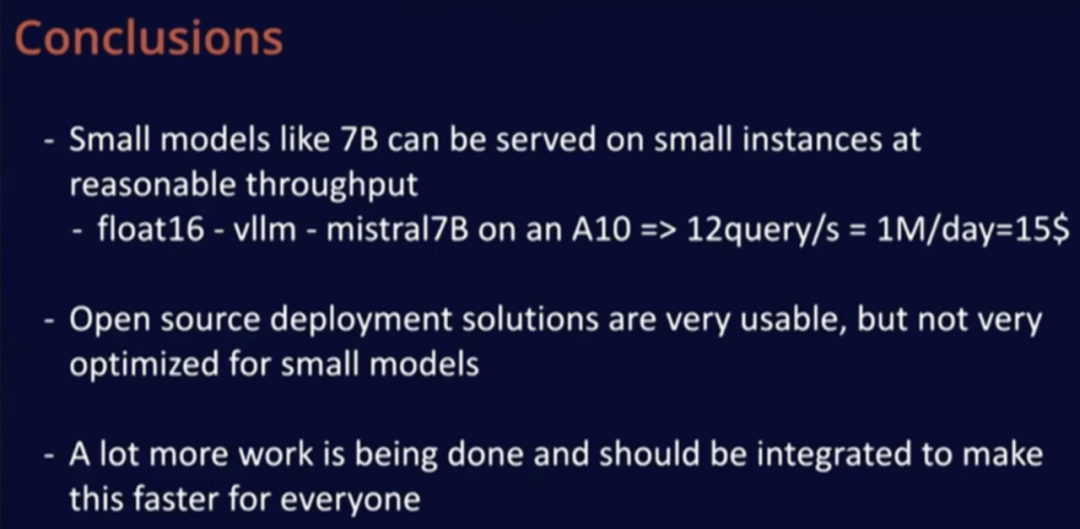
Overall, using open-source code to deploy small models on small instances is very easy, achieving good operational results without any extra operations. For about $15/day (not too high a cost), we can use the Mistral-7B model on A10 to handle millions of requests. Changing model precision could double the number of requests served.
Open-source deployment solutions perform excellently in terms of ease of use, and I believe there is still much work to be done in the actual model code part. Additionally, I believe that the speed of future models will continue to increase.
4
Answering Audience Questions
Question 1: How to choose the best processor for a specific model?
Timothée Lacroix: I have not yet tested dedicated AI hardware; I mainly tested a range of GPUs. I haven’t even run the model on a MacBook yet because I haven’t found a suitable use case, but I might try it later. For users, if you just want to chat with the model, running it directly on a MacBook is more economical. When the requests per day reach a million, using A10 is very cost-effective, at about $15 a day; if the user can afford this, I recommend choosing the A10 processor, which is easy to deploy and performs well.
Regarding the choice of hardware scale, since hardware is easy to deploy anywhere, we can start with the cheapest hardware, and if the required throughput or speed is not achieved, then consider upgrading.
I mentioned that in terms of cost, compared to using a bunch of A10 processors, H100 is a wiser choice. However, we often face availability issues. Therefore, I suggest trying them one by one in order of processor cost and availability. If you try these processors for about 20 minutes, the cost of doing so is relatively low, and this is roughly the longest time required to run a benchmark. This way, you can obtain accurate cost and performance data for specific use cases in a short time, allowing you to better choose the processor that fits your needs.
Question 2: Do you recommend using Mojo to reduce Python overhead? Have you tried using Mojo?
Timothée Lacroix: Not at all. My first attempt to reduce overhead was through CUDA graphs; although there were some difficulties during debugging, things have improved over time, and XFormers is a great example. In the future, torch.compile may effectively reduce Python overhead, but I am not clear on their progress in handling variable sequence lengths and so on. In summary, I highly recommend CUDA graphs, which is my current preferred method for reducing overhead.
Question 3: If we want LLM to have multilingual understanding capabilities, but currently the dataset is mainly in English, and the effect of fine-tuning with non-English data is not ideal, what is the most effective strategy for this situation?
Timothée Lacroix: All capabilities of LLM come from data, so we first need to obtain data in the target language. All LLMs are trained on Wikipedia, which lays a good foundation for the model to master multilingual capabilities; this also explains why the model can understand some French without special training. I think there is a trade-off in getting the model to master multilingual capabilities; for example, if the model makes progress in French, it will slightly lose capabilities in other languages, but this loss is not significant and is acceptable, as overall performance improvements in other languages may be more pronounced.
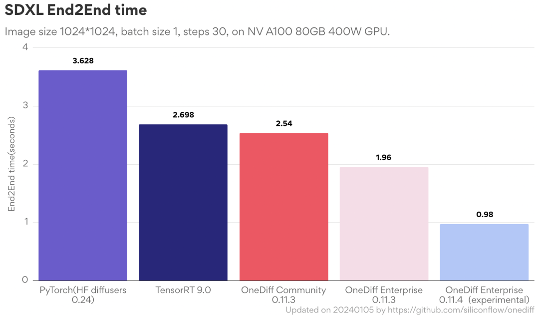
OneDiff is an out-of-the-box image/video generation inference engine. Latest features of the open-source version: 1. Switch image sizes without recompilation (i.e., no time consumption); 2. Save and load images faster; 3. Smaller static memory.
Address: https://github.com/siliconflow/onediff
Usage: https://github.com/siliconflow/onediff/releases/tag/0.12.0
-
800+ Page Free “Large Model” eBook
-
Inference Techniques for Large Language Models
-
Inference Calculation of Large Language Models
-
Is Scaling Large Models Sustainable?
-
Reproducible Inference Performance Metrics for Large Language Models
-
Performance Engineering for Large Language Model Inference: Best Practices
-
Towards 100x Speedup: Full-Stack Transformer Inference Optimization
Try OneDiff: github.com/siliconflow/onediff
800+ Page Free “Large Model” eBook
Inference Techniques for Large Language Models
Inference Calculation of Large Language Models
Is Scaling Large Models Sustainable?
Reproducible Inference Performance Metrics for Large Language Models
Performance Engineering for Large Language Model Inference: Best Practices
Towards 100x Speedup: Full-Stack Transformer Inference Optimization