Click on “Computer Vision Life” above, and select “Star”
Quickly get the latest insights
This article is compiled from Zhihu Q&A. If there is any infringement, please delete it.
Editor丨Extreme City Platform
I think the most enlightening work for me is by Xu Zhiqin from Shanghai Jiao Tong University.
https://ins.sjtu.edu.cn/people/xuzhiqin/fprinciple/index.html
https://www.bilibili.com/video/av94808183?p=2
Additionally, I have attended his talks offline about neural networks and Fourier transforms, almost all focused on these topics.
Training behavior of deep neural network in frequency domain
https://arxiv.org/pdf/1807.01251.pdf
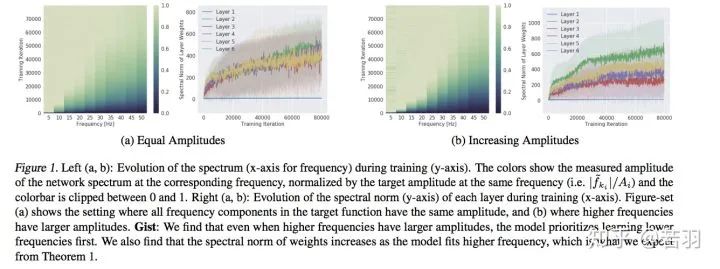
This paper explicitly states that the generalization performance of neural networks stems from their training process, which focuses more on low-frequency components.
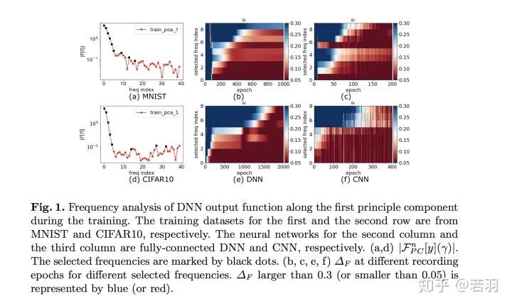
The fitting process of neural networks for CIFAR-10 and MNIST, where blue represents low frequency and red represents high frequency, shows that as training approaches convergence, fewer low-frequency components need to be learned.
Theory of the frequency principle for general deep neural networks
https://arxiv.org/pdf/1906.09235v2.pdf
A large amount of mathematical derivation is done to prove the F-Principle, dividing the proof into initial, intermediate, and final training phases, which can be a bit cumbersome for non-mathematics majors.
Explicitizing an Implicit Bias of the Frequency Principle in Two-layer Neural Networks
https://arxiv.org/pdf/1905.10264.pdf
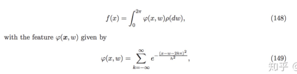
Why deep neural networks (DNNs) with more parameters than samples often generalize well remains a mystery. One attempt to understand this issue is to discover the implicit bias during DNNs training, such as the frequency principle (F-Principle), which states that DNNs typically fit target functions from low frequency to high frequency. Inspired by the F-Principle, this paper proposes an effective linear F-Principle dynamics model that accurately predicts the learning outcomes of wide two-layer ReLU neural networks (NNs). This Linear FP dynamics is rationalized by the linearized Mean Field residual dynamics of NNs. Importantly, the long-time limit solution of this LFP dynamics is equivalent to the solution of a constrained optimization problem that explicitly minimizes the FP norm, where feasible solutions are penalized more severely for high frequencies. Using this optimization formula, a prior estimate of the generalization error bound is provided, indicating that the higher the FP norm of the target function, the greater the generalization error. Overall, by interpreting the implicit bias of the F-Principle as an explicit penalty for two-layer NNs, this work makes progress towards quantitatively understanding the learning and generalization of general DNNs.
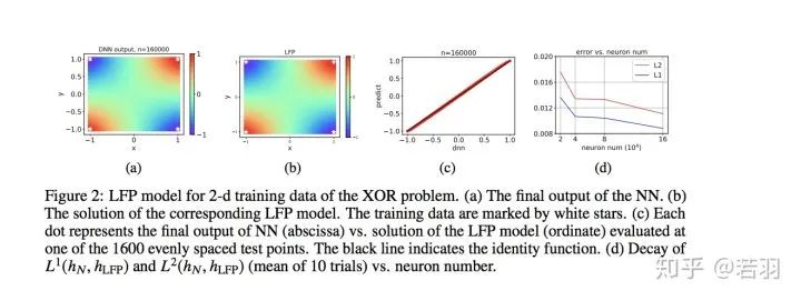
This is a schematic diagram of the LFP model for two-dimensional data in images.
Professor Xu’s previous introduction:
The LFP model provides a new perspective for the quantitative understanding of neural networks. First, the LFP model effectively characterizes the key features of the training process of a system with many parameters using a simple differential equation, and can accurately predict the learning outcomes of neural networks. Therefore, this model establishes a relationship between differential equations and neural networks from a new angle. Since differential equations are a well-established research area, we believe that tools from this field can help us further analyze the training behaviors of neural networks. Second, similar to statistical physics, the LFP model is only related to some macroscopic statistical quantities of the network parameters, rather than the specific behavior of individual parameters. This statistical characterization can help us accurately understand the learning process of DNNs when there are many parameters, thus explaining the good generalization ability of DNNs when the number of parameters far exceeds the number of training samples. In this work, we analyze the evolution results of this LFP dynamics through an equivalent optimization problem and provide a prior estimate of the network’s generalization error. We find that the generalization error of the network can be controlled by a certain F-principle norm of the target function f, which is defined as  It is worth noting that our error estimate targets the learning process of the neural network itself and does not require adding extra regularization terms in the loss function. We will further elaborate on this error estimate in subsequent articles.
FREQUENCY PRINCIPLE: FOURIER ANALYSIS SHEDS LIGHT ON DEEP NEURAL NETWORKS
https://arxiv.org/pdf/1901.06523.pdf
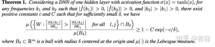
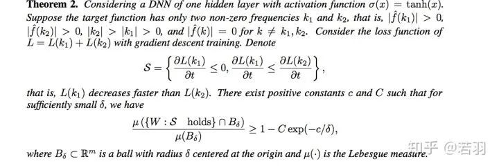
This indicates that for any two non-converging frequencies, low-frequency gradients outperform high-frequency gradients exponentially under smaller weights. According to Parseval’s theorem, the MSE loss in the spatial domain is equivalent to the L2 loss in the Fourier domain. To intuitively understand the high decay rate of the low-frequency loss function, we consider training in the Fourier domain of a loss function with only two non-zero frequencies.
Explaining why the ReLU function works, because the tanh function is smooth in the spatial domain, and its derivative decays exponentially with frequency in the Fourier region.
Professor Xu’s popular science articles on the F-Principle:
https://zhuanlan.zhihu.com/p/42847582
https://zhuanlan.zhihu.com/p/72018102
https://zhuanlan.zhihu.com/p/56077603
https://zhuanlan.zhihu.com/p/57906094
On the Spectral Bias of Deep Neural Networks
The work of the Bengio group, previously I had written a rough analysis note:
https://zhuanlan.zhihu.com/p/160806229
1. Analyzing the Fourier spectral components of ReLU networks using a continuous piecewise linear structure.
2. Finding empirical evidence of spectral bias sourced from low-frequency components, however, learning low-frequency components helps the network’s robustness against interference.
3. Providing a learning theoretical framework analysis through manifold theory.
According to the topological Stokes theorem, proving that the ReLU function is compact and smooth, aiding the convergence of training, what about the subsequent Swish and Mish? (Dog head).
Thus, in high-dimensional space, the spectral decay of the ReLU function has a strong anisotropy, and the upper limit of the amplitude of the ReLU Fourier transform satisfies the Lipschitz constraint.
Center point: The learning priority for low-frequency components is high
It is worth noting that our error estimate targets the learning process of the neural network itself and does not require adding extra regularization terms in the loss function. We will further elaborate on this error estimate in subsequent articles.
FREQUENCY PRINCIPLE: FOURIER ANALYSIS SHEDS LIGHT ON DEEP NEURAL NETWORKS
https://arxiv.org/pdf/1901.06523.pdf
This indicates that for any two non-converging frequencies, low-frequency gradients outperform high-frequency gradients exponentially under smaller weights. According to Parseval’s theorem, the MSE loss in the spatial domain is equivalent to the L2 loss in the Fourier domain. To intuitively understand the high decay rate of the low-frequency loss function, we consider training in the Fourier domain of a loss function with only two non-zero frequencies.
Explaining why the ReLU function works, because the tanh function is smooth in the spatial domain, and its derivative decays exponentially with frequency in the Fourier region.
Professor Xu’s popular science articles on the F-Principle:
https://zhuanlan.zhihu.com/p/42847582
https://zhuanlan.zhihu.com/p/72018102
https://zhuanlan.zhihu.com/p/56077603
https://zhuanlan.zhihu.com/p/57906094
On the Spectral Bias of Deep Neural Networks
The work of the Bengio group, previously I had written a rough analysis note:
https://zhuanlan.zhihu.com/p/160806229
1. Analyzing the Fourier spectral components of ReLU networks using a continuous piecewise linear structure.
2. Finding empirical evidence of spectral bias sourced from low-frequency components, however, learning low-frequency components helps the network’s robustness against interference.
3. Providing a learning theoretical framework analysis through manifold theory.
According to the topological Stokes theorem, proving that the ReLU function is compact and smooth, aiding the convergence of training, what about the subsequent Swish and Mish? (Dog head).
Thus, in high-dimensional space, the spectral decay of the ReLU function has a strong anisotropy, and the upper limit of the amplitude of the ReLU Fourier transform satisfies the Lipschitz constraint.
Center point: The learning priority for low-frequency components is high
-
Experimenting on functions:

Fourier transform effects
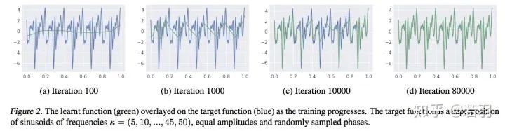
Iterative process of function learning
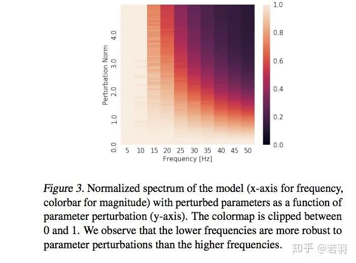
Standardized spectral components of the model
2. Learning MNIST data in a noisy environment
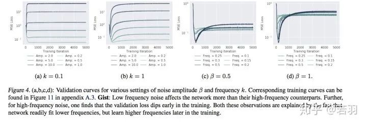
Different validation losses
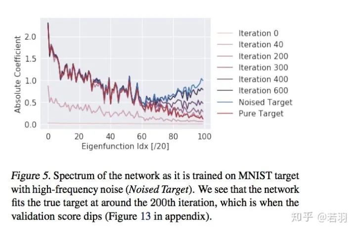
Frequency components of MNIST data fitting
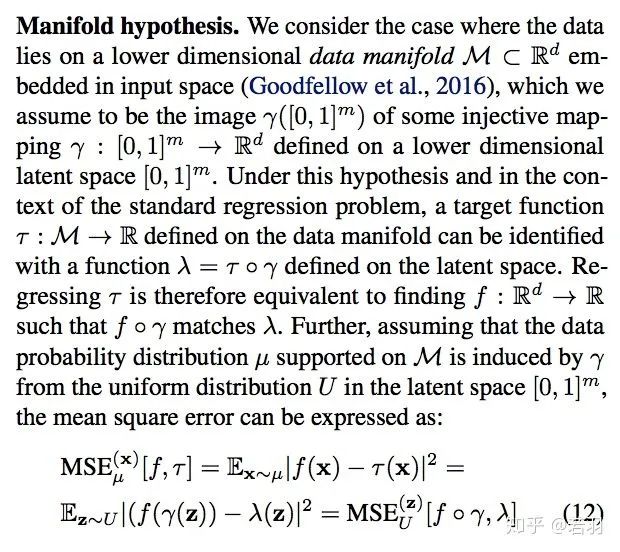
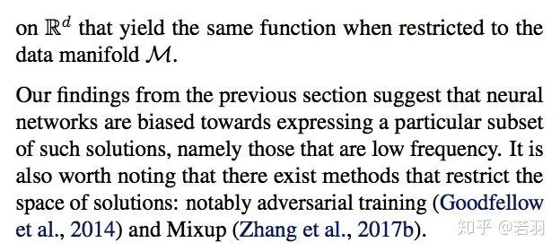
Neural networks can approximate any value function, but researchers found they prefer low-frequency components, thus exhibiting a bias towards smooth functions—a phenomenon known as spectral bias.
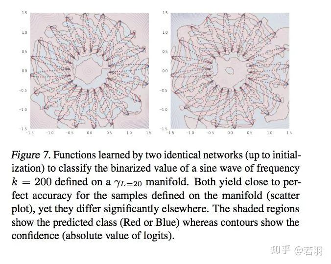
The more complex the manifold, the easier the learning process becomes; this hypothesis may break the “structural risk minimization” assumption, potentially leading to “overfitting”.
If there are complex datasets (like ImageNet), the search space is relatively large, and certain methods must be employed to ensure they “work in harmony” and operate in a tuned manner.
It seems Bengio believes this has enlightening implications for regularization in deep learning.
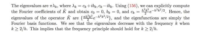
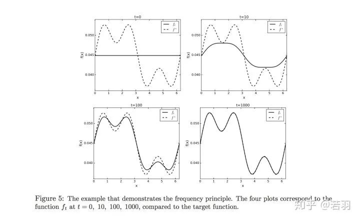
Machine Learning from a Continuous Viewpoint
https://arxiv.org/pdf/1912.12777.pdf
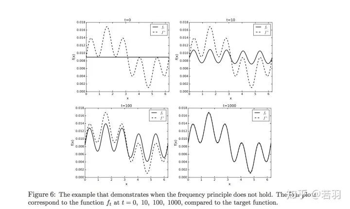
Mathematician Wienan.E’s contention that the frequency principle does not always work.
Assuming a certain function:
 Probability measure
Based on kernel functions for derivation:
Performing Fourier coefficient decomposition:
Then the boundaries of when the frequency principle works are given.
Conditions under which it works:
Conditions under which it does not work:
If Wienan. E provided the boundaries of the Frequency Principle from a mathematician’s perspective, then engineering colleagues must check this paper:
A Fourier Perspective on Model Robustness in Computer Vision
https://arxiv.org/pdf/1906.08988.pdf
The code has also been open-sourced:
https://github.com/google-research/google-research/tree/master/frequency_analysis
The author’s intention is to focus on robustness, without completely discarding high-frequency features.
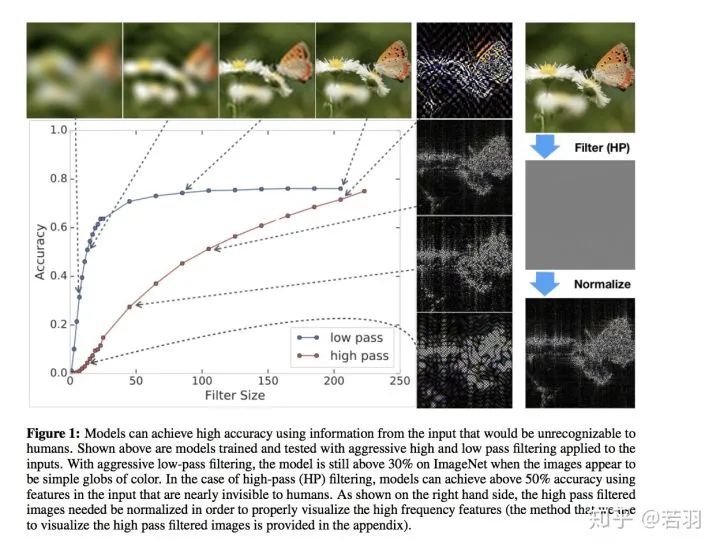
Image description translation: Using input information that humans cannot recognize, the model can achieve high accuracy. The above shows the trained and tested models, which applied strict high-pass and low-pass filtering at the input end. Through positive low-pass filtering, when the image appears as a simple colored sphere, the model still exceeds 30% accuracy on ImageNet. In the case of high-pass (HP) filtering, using input features that are almost invisible to humans, the model can achieve over 50% accuracy. As shown on the right, normalization is needed for high-pass filtered images to correctly visualize high-frequency features (we use the method provided in the appendix to visualize the high-pass filtered images).
Probability measure
Based on kernel functions for derivation:
Performing Fourier coefficient decomposition:
Then the boundaries of when the frequency principle works are given.
Conditions under which it works:
Conditions under which it does not work:
If Wienan. E provided the boundaries of the Frequency Principle from a mathematician’s perspective, then engineering colleagues must check this paper:
A Fourier Perspective on Model Robustness in Computer Vision
https://arxiv.org/pdf/1906.08988.pdf
The code has also been open-sourced:
https://github.com/google-research/google-research/tree/master/frequency_analysis
The author’s intention is to focus on robustness, without completely discarding high-frequency features.
Image description translation: Using input information that humans cannot recognize, the model can achieve high accuracy. The above shows the trained and tested models, which applied strict high-pass and low-pass filtering at the input end. Through positive low-pass filtering, when the image appears as a simple colored sphere, the model still exceeds 30% accuracy on ImageNet. In the case of high-pass (HP) filtering, using input features that are almost invisible to humans, the model can achieve over 50% accuracy. As shown on the right, normalization is needed for high-pass filtered images to correctly visualize high-frequency features (we use the method provided in the appendix to visualize the high-pass filtered images).
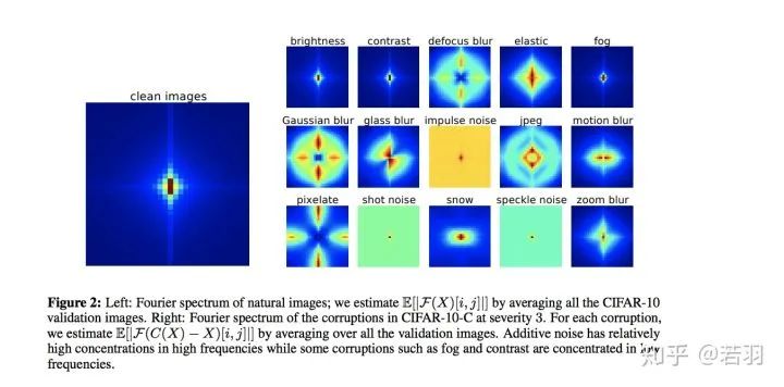 Image description translation: Left: Fourier spectrum of natural images; we estimate E[|F(X)[i,j]|] by averaging all CIFAR-10 validation images. Right: Fourier spectrum of corruption severity 3 in CIFAR-10-C. For each corruption, we estimate E[|F(C(X)−X)[i,j]|] by averaging all validation images. Additive noise has a higher concentration in the high-frequency band, while fog, contrast, etc., are concentrated in the low-frequency band.
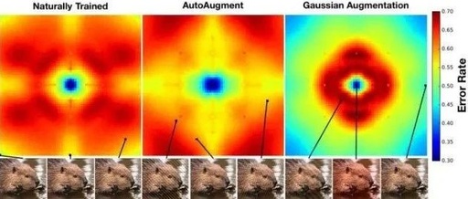
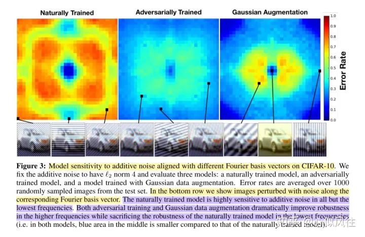
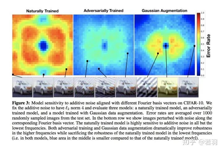 Image translation explanation: Model sensitivity to additive noise from different Fourier basis vectors on CIFAR-10. We fixed the additive noise to “L2 norm = 4” and evaluated three models: naturally trained model, adversarially trained model, and Gaussian data-augmented trained model. We averaged the error rates from 1000 random samples of images from the test set. In the bottom row, we show images disturbed by noise along the corresponding Fourier basis vectors. The naturally trained model is highly sensitive to all additive noise except the lowest frequency. Both adversarial training and Gaussian data augmentation significantly improve robustness at high frequencies while sacrificing the robustness of the naturally trained model at low frequencies (i.e., in these two models, the middle blue area is smaller than in the naturally trained model).
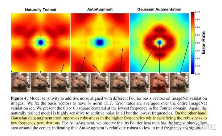
 Image translation explanation: Sensitivity of different Fourier basis vectors to additive noise on ImageNet validation images. We fixed the basis vector to an L2 norm value of 15.7. The error rate is the average error rate across the entire ImageNet validation set. A 63×63 square centered on the lowest frequency in the Fourier domain is provided. Similarly, the naturally trained model is highly sensitive to all additive noise except the lowest frequency. On the other hand, Gaussian data augmentation improves robustness at high frequencies while sacrificing robustness against low-frequency disturbances. For AutoAugment, we observe that its Fourier heatmap has the largest blue/yellow area around the center, indicating that AutoAugment is relatively robust against low to mid-frequency destruction.
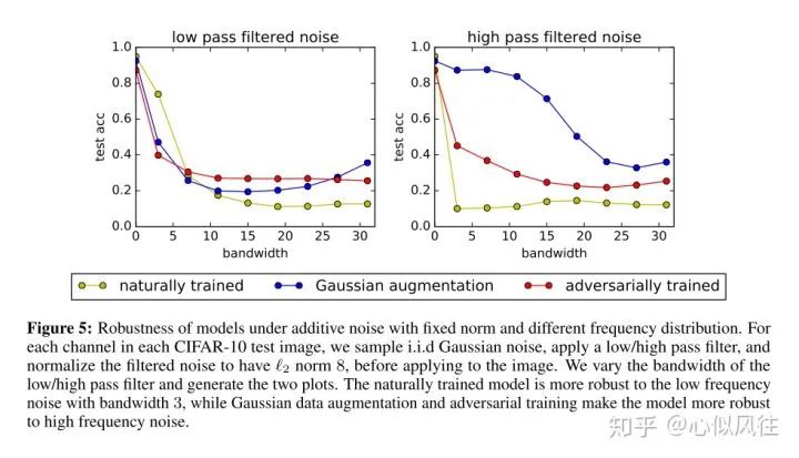
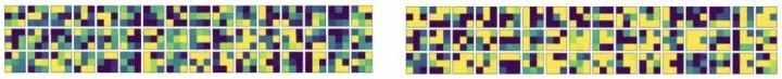 Image translation explanation: Robustness of the model under additive noise with fixed norm and different frequency distributions. For each channel in each CIFAR-10 test image, we sample independent identically distributed Gaussian noise, apply low/high-pass filters, and normalize the filtered noise to an L2 norm value of 8 before applying it to the image. We change the bandwidth of the low/high-pass filters to generate two curves. The naturally trained model exhibits greater robustness against low-frequency noise with a bandwidth of 3, while Gaussian data augmentation and adversarial training enhance the model’s robustness against high-frequency noise.
 Image translation explanation: Relationship between the frequency energy fraction of CIFAR-10-C corruption and test accuracy. Each scatter point in the plot represents the evaluation results of a specific model against a specific type of corruption. The X-axis represents the score of high-frequency energy of the corruption type, while the Y-axis represents the change in test accuracy compared to the naturally trained model. Overall, Gaussian data augmentation, adversarial training, and adding low-pass filters improve robustness against high-frequency corruption while reducing robustness against low-frequency corruption. Applying high-pass filters results in a more significant accuracy drop for high-frequency corruption than for low-frequency corruption. AutoAugment improves robustness against nearly all corruptions and achieves the best overall performance. The legend at the bottom shows the slope (K) and residual (r) of each fitted line.
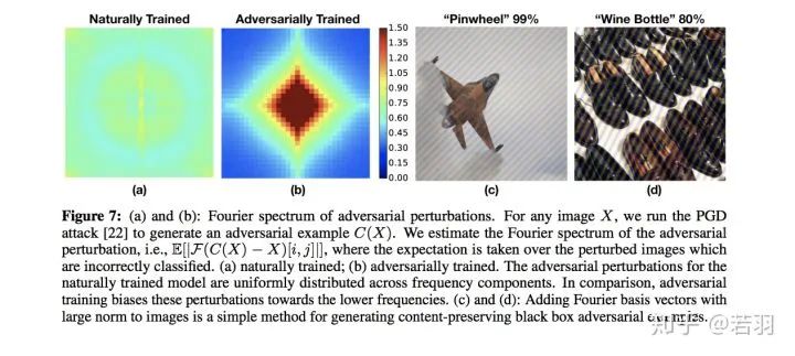 Image translation explanation: (a) and (b): Fourier spectra of adversarial perturbations. Given image X, initiating a PGD attack yields adversarial sample C(X), estimating the Fourier spectrum of the adversarial perturbation that causes incorrect classification of the image; (a) is the spectrum obtained from natural training; (b) is the spectrum obtained from adversarial training. The adversarial perturbations of the naturally trained model are uniformly distributed across frequency components. In contrast, adversarial training biases these perturbations towards lower frequencies. (C) and (D): Adding Fourier basis vectors with large norms to the image is a simple method to generate content-preserving adversarial examples in a black box manner.
1) Adversarial training focuses on some high-frequency components rather than obsessively fixating on low-frequency components.
2) AutoAugment helps improve robustness.
The open-source code mainly teaches how to draw similar schematic diagrams as in the paper.
Additionally, there is another paper from Eric Xing’s group, which has been previously published by Zhihu’s self-media:
High-frequency Component Helps Explain the Generalization of Convolutional Neural Networks
https://arxiv.org/pdf/1905.13545.pdf
Visualization of convolutions from natural training and adversarial training
The paper experimented with several methods:
Image translation explanation: (a) and (b): Fourier spectra of adversarial perturbations. Given image X, initiating a PGD attack yields adversarial sample C(X), estimating the Fourier spectrum of the adversarial perturbation that causes incorrect classification of the image; (a) is the spectrum obtained from natural training; (b) is the spectrum obtained from adversarial training. The adversarial perturbations of the naturally trained model are uniformly distributed across frequency components. In contrast, adversarial training biases these perturbations towards lower frequencies. (C) and (D): Adding Fourier basis vectors with large norms to the image is a simple method to generate content-preserving adversarial examples in a black box manner.
1) Adversarial training focuses on some high-frequency components rather than obsessively fixating on low-frequency components.
2) AutoAugment helps improve robustness.
The open-source code mainly teaches how to draw similar schematic diagrams as in the paper.
Additionally, there is another paper from Eric Xing’s group, which has been previously published by Zhihu’s self-media:
High-frequency Component Helps Explain the Generalization of Convolutional Neural Networks
https://arxiv.org/pdf/1905.13545.pdf
Visualization of convolutions from natural training and adversarial training
The paper experimented with several methods:
-
For a trained model, we adjust its weights to smooth the convolution kernels;
-
Directly filtering out high-frequency information from the trained convolution kernels;
-
Adding regularization during the training of convolutional neural networks to make the weights of adjacent positions closer.
Focusing on low-frequency information helps improve generalization; high-frequency components may be related to adversarial attacks, but one should not be too dogmatic.
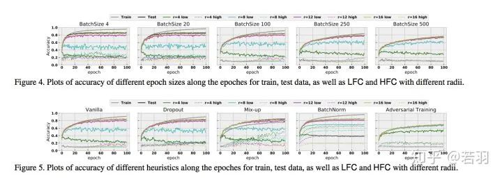
The contribution is to provide detailed experimental evidence that Batch Normalization is useful for fitting high-frequency components and improving generalization.
Finally, it’s all just talk.
On this side, Professor Xu proves that the smoothness of ReLU aids function optimization; on the other side, a recent work called Bandlimiting Neural Networks Against Adversarial Attacks
https://arxiv.org/pdf/1905.12797.pdf
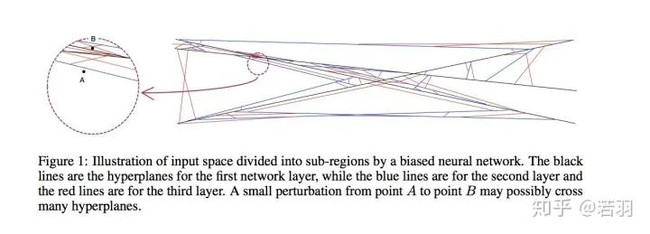
ReLU function obtains a piecewise linear function
Can be decomposed into numerous frequency components.
For N=1000 hidden layer nodes and input dimension n=200, the maximum number of regions is approximately equal to 10^200. In other words, even a moderately sized neural network can partition the input space into a vast number of sub-regions, easily exceeding the total number of atoms in the universe. When we learn neural networks, we cannot expect that there is at least one sample in every region. For those regions without any training samples, the resulting linear functions can be arbitrary since they do not contribute to the training target function at all. Of course, most of these regions are very small. When we measure the expected loss function across the entire space, their contribution can be negligible because the chance of random sampling points falling into these tiny regions is very small. However, adversarial attacks present new challenges, as adversarial samples are not naturally sampled. Considering the total number of regions is enormous, these tiny regions are almost everywhere in the input space. For any data point in the input space, we can almost certainly find such a tiny region where the linear function is arbitrary. If a point within this tiny region is chosen, the output of the neural network may be unexpected. These tiny regions are the fundamental reason neural networks are vulnerable to adversarial attacks.
Then, a method of adversarial defense is proposed, which I couldn’t understand; readers can read the paper themselves, and I welcome any pointers in the comments after reading.
Although I have procrastination, I will share other related and interesting papers when I come across them.
https://www.zhihu.com/question/59532432/answer/1510340606
Author丨Heart Like the Wind
After receiving the invitation, I followed this question for a while, thinking that if someone answered it seriously, I could save time and get the answer for free, secretly pleased. However, after waiting a long time, no one answered it carefully. I could only step up and throw a brick to attract jade.
It’s quite miraculous that I happened to read an article about understanding and analyzing model robustness from the frequency domain, and part of its content coincidentally analyzed this issue, and very coincidentally: the experiments also used ResNet. Isn’t that a coincidence!
First, let me post the name of the paper:
A Fourier Perspective on Model Robustness in Computer Vision [1]
First of all, deep learning models have achieved unprecedented success, but there is a significant problem, which is their poor robustness; that is, adding a little corruption to certain test images can lead to incorrect classification. One method to enhance robustness is to perform data augmentation on the training set images, allowing the trained model to resist corruption. However, the author found that the same data augmentation methods such as Gaussian augmentation and adversarial training do not improve robustness for all corruption scenarios. Therefore, the author raised the question: Why do the same augmentation methods improve performance for some corruptions while reducing performance for others?
Then, the author proposed a hypothesis: Could it be that different corruptions provide different frequency information?
For CIFAR-10, the author used Wide ResNet-28-10;
For ImageNet, the author used ResNet-50.
The author analyzed the impact of different frequency information in images on the prediction accuracy of naturally trained models.
As shown in the figure above, the author conducted experiments with the ResNet-50 model trained on ImageNet.
For low-frequency information, the author directly added low-pass filters in the frequency domain of the test images, allowing different amounts of low-frequency signals to pass through based on the size of the filters, with four typical filtered images displayed above the chart.
For high-frequency information, the author added high-pass filters in the frequency domain of the images and performed normalization. Different filter sizes allowed varying amounts of high-frequency signals to pass through, with four typical filtered images displayed on the right side of the chart.
The x-axis of the chart represents the size of the filter, while the y-axis represents classification accuracy.
The chart above indicates that even when the low-pass filter is very small, and the image looks like a color block that the human eye cannot distinguish, the model still achieves over 30% accuracy (the first image derived from the low-pass filter). For the high-pass filtered part (the second image from the top), even when the human eye cannot distinguish what is in the image, the model still achieves 50% accuracy. Furthermore, when low-frequency information is scarce, increasing low-frequency information can quickly improve accuracy, and once a certain amount is reached, it no longer affects accuracy; the impact of high-frequency information on accuracy gradually increases, without being as rapid as low frequency.
With CIFAR-10 as the training set, the author analyzed the sensitivity of the Wide ResNet-28-10 model to additive noise.
The center of the image is the low-frequency signal area, with increasing frequency towards the edges.
With CIFAR-10 as the training set, the trained model is Wide ResNet-28-10.
The naturally trained model is sensitive to all frequencies except low-frequency corruption noise, while adversarial training and Gaussian augmentation improve the model’s robustness against high-frequency corruption (lower error rates).
With ImageNet as the training set, the author analyzed the sensitivity of the ResNet-50 model to additive noise.
The naturally trained model is sensitive to all frequencies except low-frequency corruption noise; Gaussian augmentation sacrifices robustness against low-frequency perturbations while enhancing robustness against high frequencies. For AutoAugment, robustness gradually decreases for low, mid, and high frequencies.
The effect of increasing bandwidth on the influence of high-frequency and low-frequency signals on test accuracy.
With CIFAR-10 as the training set, the model is Wide ResNet-28-10.
Compared to the naturally trained model, as the noise filter bandwidth increases, test accuracy decreases, while we find that the accuracy of the models obtained through Gaussian augmentation and adversarial training is higher than that of the naturally trained model.
Supplement 1:According to @Lost’s answer to this question, I also recommend everyone to read the paper he mentioned: Frequency Principle: Fourier Analysis Sheds Light on Deep Neural Networks[2]
https://arxiv.org/pdf/1901.06523.pdf
Supplement 2:Also recommend everyone to read the following paperHigh-frequency Component Helps Explain the Generalization of Convolutional Neural Network[3]
https://openaccess.thecvf.com/content_CVPR_2020/papers/Wang_High-Frequency_Component_Helps_Explain_the_Generalization_of_Convolutional_Neural_Networks_CVPR_2020_paper.pdf
[1] A Fourier Perspective on Model Robustness in Computer Vision
[2] Frequency Principle: Fourier Analysis Sheds Light on Deep Neural Networks
[3] High-frequency Component Helps Explain the Generalization of Convolutional Neural Network
https://www.zhihu.com/question/59532432/answer/1447173834
Album: Introduction to Computer Vision Direction
Album: Introduction to Visual SLAM
Album: Latest SLAM/3D Vision Papers/Open Source
Album: 3D Vision/SLAM Open Courses
Album: Principles and Applications of Depth Cameras
Album: Analysis and Applications of Dual Camera Technology on Mobile Phones
Album: Camera Calibration
Album: Panoramic Cameras
Group Chat
Welcome to join the WeChat reader group for exchanges with peers. Currently, there are WeChat groups for SLAM、三维视觉、传感器、自动驾驶、计算摄影、检测、分割、识别、医学影像、GAN、算法竞赛等微信群(以后会逐渐细分),请扫描下面微信号加群,备注:”昵称+学校/公司+研究方向“,例如:”张三 + 上海交大 + 视觉SLAM“。请按照格式备注,否则不予通过。添加成功后会根据研究方向邀请进入相关微信群。请勿在群内发送广告,否则会请出群,谢谢理解~
Submissions and collaborations are also welcome:[email protected]

Scan to follow the video account and see the latest technology implementation and open-source solution video showcase ↓