↑ ClickBlue Text Follow the Jishi Platform
This article is authorized by Zhihu Q&A, reprinting requires authorization from the original author.
How to think about and explain convolutional neural networks from the perspective of the frequency domain? This article整理了两则优质回答,希望能给大家带来启发。>> Join the Jishi CV technology exchange group and stay at the forefront of computer vision
I think the most enlightening work for me is by Xu Zhiqin from Shanghai Jiao Tong University.
https://ins.sjtu.edu.cn/people/xuzhiqin/fprinciple/index.html
https://www.bilibili.com/video/av94808183?p=2
In addition, I have heard him speak offline about twice, almost all regarding the work on neural networks and Fourier transforms, Fourier analysis.
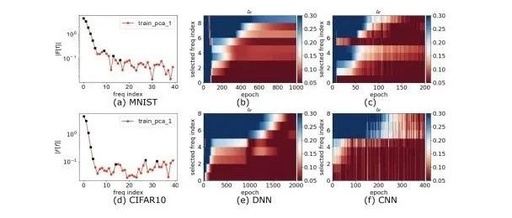
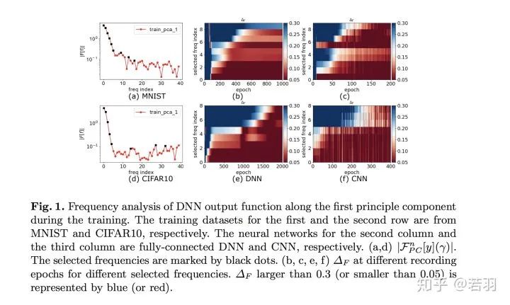
Training behavior of deep neural network in frequency domain
https://arxiv.org/pdf/1807.01251.pdf
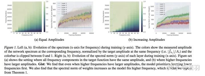
This paper explicitly states that the generalization performance of neural networks comes from their training process, which focuses more on low-frequency components.
The fitting process of neural networks for CIFAR-10 and MNIST, with blue representing low-frequency and red representing high-frequency, shows that as the training approaches convergence, the low-frequency components that need to be learned decrease.
Theory of the frequency principle for general deep neural networks
https://arxiv.org/pdf/1906.09235v2.pdf
Extensive mathematical derivation is done to prove the F-Principle, dividing the training into initial, intermediate, and final stages for proof, which can be a bit cumbersome for non-mathematics majors.
Explicitizing an Implicit Bias of the Frequency Principle in Two-layer Neural Networks
https://arxiv.org/pdf/1905.10264.pdf
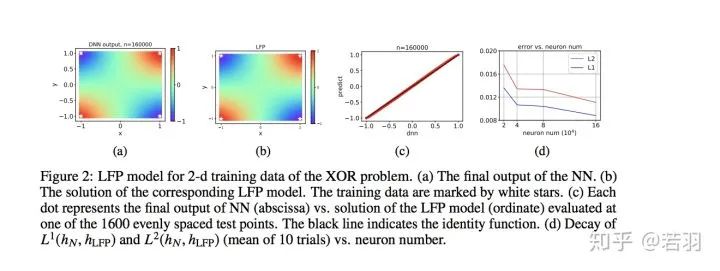
Why deep neural networks (DNNs) with more parameters than samples can often generalize well remains a mystery. One attempt to understand this issue is to discover the implicit bias in the training process of DNNs, such as the frequency principle (F-Principle), which states that DNNs typically fit target functions from low to high frequencies. Inspired by the F-Principle, this paper proposes an effective linear F-Principle dynamic model that accurately predicts the learning outcomes of wide two-layer ReLU neural networks (NNs). This Linear FP dynamic is rationalized by the linearized Mean Field residual dynamics of NNs. Importantly, the long-time limit solution of this LFP dynamic is equivalent to the solution of an explicit optimization problem that minimizes the FP norm under constraints, where feasible solutions are more severely penalized for high frequencies. Using this optimization formula, a prior estimate of the generalization error bound is provided, indicating that the higher the FP norm of the target function, the greater the generalization error. Overall, by interpreting the implicit bias of the F-Principle as an explicit penalty for two-layer NNs, this work makes progress toward quantitatively understanding the learning and generalization of general DNNs.
This is a schematic diagram of the LFP model for two-dimensional data in images.
Professor Xu’s previous introduction:
The LFP model provides a new perspective for the quantitative understanding of neural networks. Firstly, the LFP model effectively characterizes the key features of the training process of a neural network, a system with numerous parameters, using a simple differential equation and can accurately predict the learning outcomes of neural networks. Therefore, this model establishes the relationship between differential equations and neural networks from a new perspective. Since differential equations are a very mature field of research, we believe that tools from this field can help us further analyze the training behavior of neural networks. Secondly, similar to statistical physics, the LFP model only relates to some macroscopic statistics of network parameters, not the specific behavior of individual parameters. This statistical characterization can help us accurately understand the learning process of DNNs when there are many parameters, thus explaining the good generalization ability of DNNs when the parameters far exceed the number of training samples. In this work, we analyze the evolution results of this LFP dynamic through an equivalent optimization problem and provide a prior estimate of the network’s generalization error. We find that the generalization error of the network can be controlled by a kind of FP norm of the target function f itself (defined as  , where γ(ξ) is a weight function that decays with frequency). It is worth noting that our error estimate targets the learning process of the neural network itself and does not require adding additional regularization terms in the loss function. We will further explain this error estimate in subsequent articles.
FREQUENCY PRINCIPLE: FOURIER ANALYSIS SHEDS LIGHT ON DEEP NEURAL NETWORKS
https://arxiv.org/pdf/1901.06523.pdf
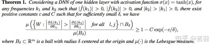
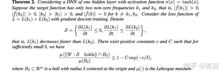
This indicates that for any two non-convergent frequencies, the low-frequency gradient exponentially outperforms the high-frequency gradient under smaller weights. According to Parseval’s theorem, the MSE loss in the spatial domain is equivalent to the L2 loss in the Fourier domain. To intuitively understand the high decay rate of the low-frequency loss function, we consider training in the Fourier domain of the loss function with only two non-zero frequencies.
It explains why the ReLU function works, as the tanh function is smooth in the spatial domain, and its derivative decays exponentially with frequency in the Fourier domain.
Professor Xu’s several popular science articles on the F-Principle:
https://zhuanlan.zhihu.com/p/42847582
https://zhuanlan.zhihu.com/p/72018102
https://zhuanlan.zhihu.com/p/56077603
https://zhuanlan.zhihu.com/p/57906094
On the Spectral Bias of Deep Neural Networks
The work by the Bengio group, I previously wrote a rough analysis note:
https://zhuanlan.zhihu.com/p/160806229
1. Analyzing the Fourier spectral components of ReLU networks using continuous piecewise linear structures.
2. Finding empirical evidence of spectral bias originating from low-frequency components, but learning low-frequency components helps the network’s robustness in adversarial processes.
3. Providing a learning theoretical framework analysis through manifold theory.
Using the topological Stokes theorem, proving that the ReLU function is compact and smooth, which helps with training convergence; what about Swish and Mish? (Dog head).
In high-dimensional space, the spectral decay of the ReLU function has strong anisotropy, and the upper limit of the amplitude of the ReLU Fourier transform satisfies the Lipschitz constraint.
Center point: High priority for learning low-frequency components
, where γ(ξ) is a weight function that decays with frequency). It is worth noting that our error estimate targets the learning process of the neural network itself and does not require adding additional regularization terms in the loss function. We will further explain this error estimate in subsequent articles.
FREQUENCY PRINCIPLE: FOURIER ANALYSIS SHEDS LIGHT ON DEEP NEURAL NETWORKS
https://arxiv.org/pdf/1901.06523.pdf
This indicates that for any two non-convergent frequencies, the low-frequency gradient exponentially outperforms the high-frequency gradient under smaller weights. According to Parseval’s theorem, the MSE loss in the spatial domain is equivalent to the L2 loss in the Fourier domain. To intuitively understand the high decay rate of the low-frequency loss function, we consider training in the Fourier domain of the loss function with only two non-zero frequencies.
It explains why the ReLU function works, as the tanh function is smooth in the spatial domain, and its derivative decays exponentially with frequency in the Fourier domain.
Professor Xu’s several popular science articles on the F-Principle:
https://zhuanlan.zhihu.com/p/42847582
https://zhuanlan.zhihu.com/p/72018102
https://zhuanlan.zhihu.com/p/56077603
https://zhuanlan.zhihu.com/p/57906094
On the Spectral Bias of Deep Neural Networks
The work by the Bengio group, I previously wrote a rough analysis note:
https://zhuanlan.zhihu.com/p/160806229
1. Analyzing the Fourier spectral components of ReLU networks using continuous piecewise linear structures.
2. Finding empirical evidence of spectral bias originating from low-frequency components, but learning low-frequency components helps the network’s robustness in adversarial processes.
3. Providing a learning theoretical framework analysis through manifold theory.
Using the topological Stokes theorem, proving that the ReLU function is compact and smooth, which helps with training convergence; what about Swish and Mish? (Dog head).
In high-dimensional space, the spectral decay of the ReLU function has strong anisotropy, and the upper limit of the amplitude of the ReLU Fourier transform satisfies the Lipschitz constraint.
Center point: High priority for learning low-frequency components
-
Experimenting with functions:

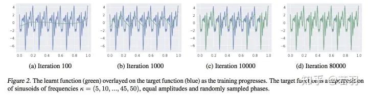
Learning of the function through iterations
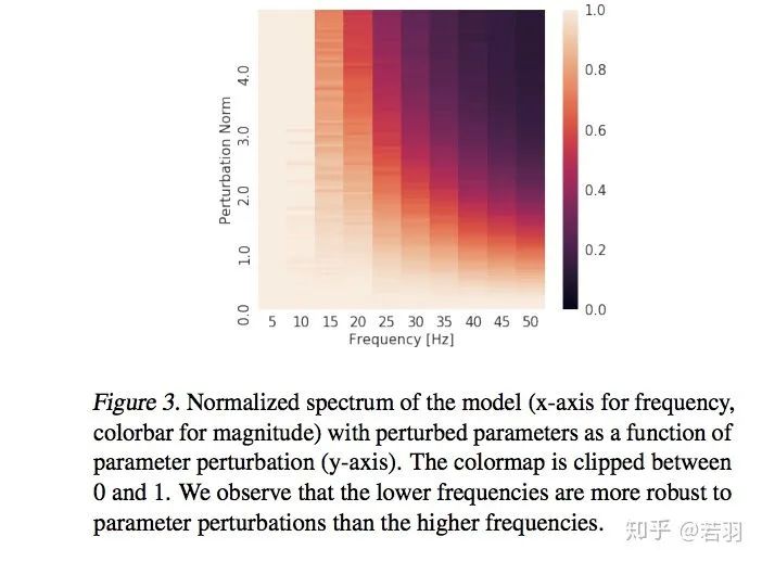
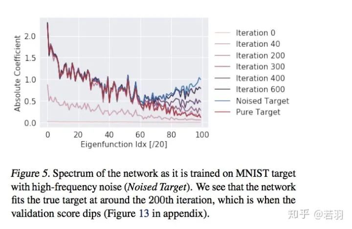
Standardized spectral components of the model
2. Learning MNIST data in a noisy environment
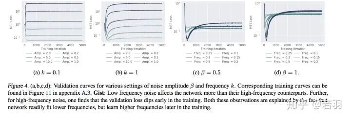
Different validation losses
Frequency components of MNIST data fitting
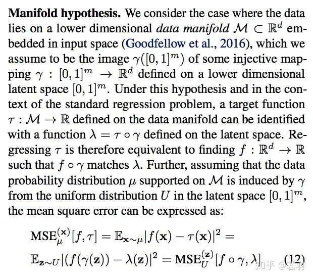
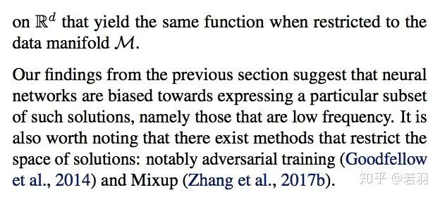
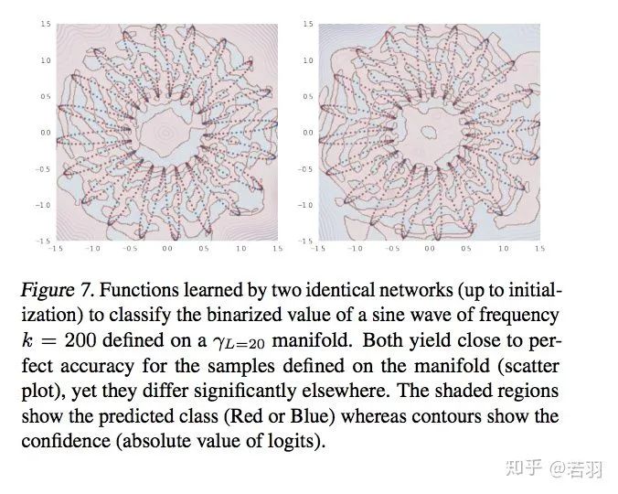
Neural networks can approximate any value function, but researchers found they prefer low-frequency components, thus exhibiting a bias toward smooth functions—a phenomenon known as spectral bias.
The more complex the manifold, the easier the learning process; this hypothesis may break the “structural risk minimization” assumption, potentially leading to “overfitting”.
If there is a complex dataset (ImageNet), the search space is relatively large, and methods must be employed to ensure it “works in harmony” and operates in a tuned manner.
It seems that Bengio believes this has implications for the regularization of deep learning.
Machine Learning from a Continuous Viewpoint
https://arxiv.org/pdf/1912.12777.pdf
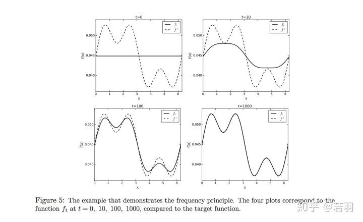
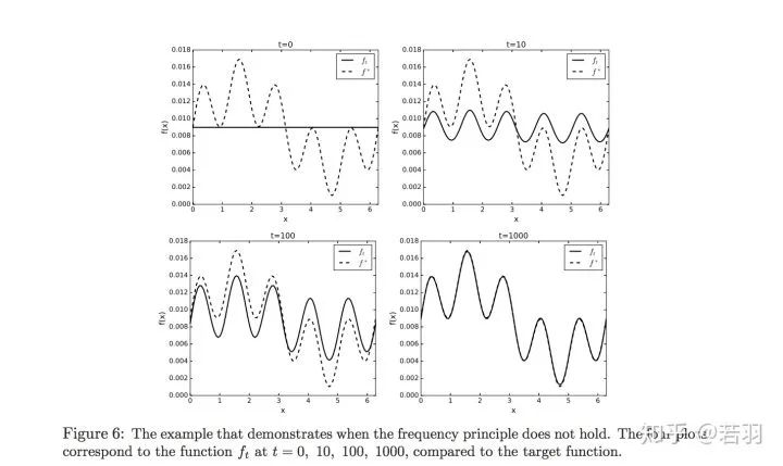
Mathematician Wienan E’s debate indicates that the frequency principle does not always work.
Assuming a certain function:
 Probability Measure
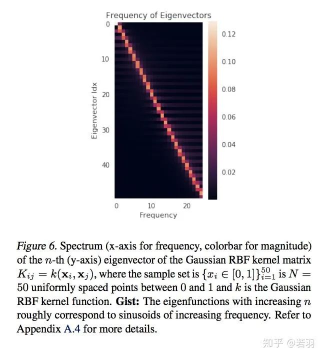
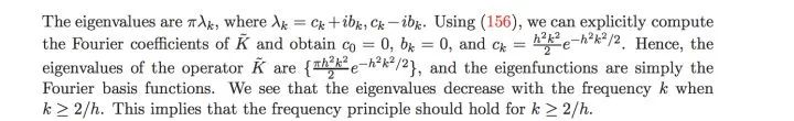
Deriving based on kernel functions:
Decomposing Fourier coefficients:
Then given the boundaries of when the frequency principle works.
Conditions under which it works:
Conditions under which it does not work:
If Wienan E provides the boundaries for the Frequency Principle from a mathematician’s perspective, then those working in engineering must certainly look at this paper:
A Fourier Perspective on Model Robustness in Computer Vision
https://arxiv.org/pdf/1906.08988.pdf
The code has also been open-sourced:
https://github.com/google-research/google-research/tree/master/frequency_analysis
The author’s intention is to focus on robustness and not completely discard high-frequency features.
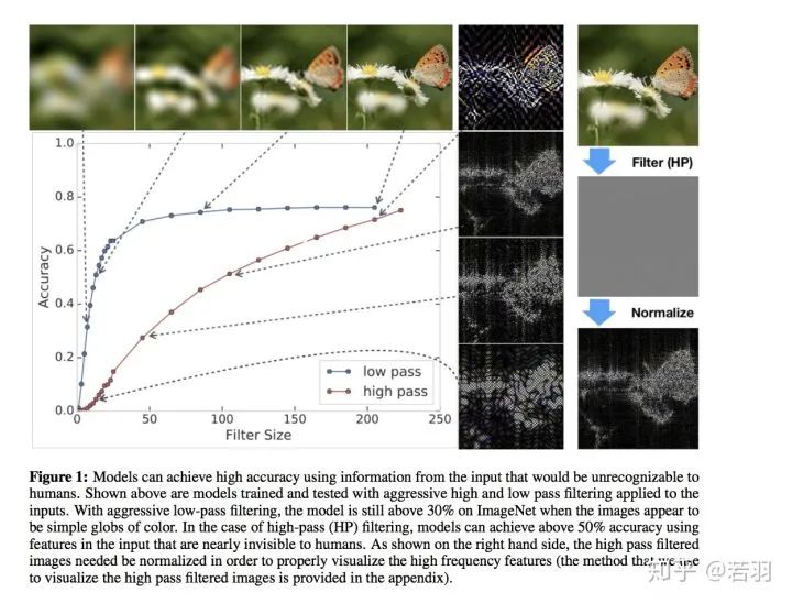
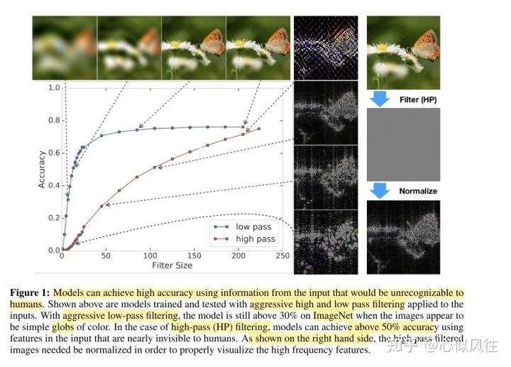
Image description translation: Using inputs that humans cannot recognize, the model can achieve high accuracy. The above shows the trained and tested models, which applied strict high-pass and low-pass filtering at the input end. Through positive low-pass filtering, when the image appears as a simple colored sphere, the model still exceeds 30% accuracy on ImageNet. In the case of high-pass (HP) filtering, using input features that are almost invisible to humans, the model can achieve over 50% accuracy. As shown on the right, high-pass filtered images need to be normalized for proper visualization of high-frequency features (we use the method provided in the appendix to visualize high-pass filtered images).
Probability Measure
Deriving based on kernel functions:
Decomposing Fourier coefficients:
Then given the boundaries of when the frequency principle works.
Conditions under which it works:
Conditions under which it does not work:
If Wienan E provides the boundaries for the Frequency Principle from a mathematician’s perspective, then those working in engineering must certainly look at this paper:
A Fourier Perspective on Model Robustness in Computer Vision
https://arxiv.org/pdf/1906.08988.pdf
The code has also been open-sourced:
https://github.com/google-research/google-research/tree/master/frequency_analysis
The author’s intention is to focus on robustness and not completely discard high-frequency features.
Image description translation: Using inputs that humans cannot recognize, the model can achieve high accuracy. The above shows the trained and tested models, which applied strict high-pass and low-pass filtering at the input end. Through positive low-pass filtering, when the image appears as a simple colored sphere, the model still exceeds 30% accuracy on ImageNet. In the case of high-pass (HP) filtering, using input features that are almost invisible to humans, the model can achieve over 50% accuracy. As shown on the right, high-pass filtered images need to be normalized for proper visualization of high-frequency features (we use the method provided in the appendix to visualize high-pass filtered images).
 Image description translation: Left: Fourier spectrum of natural images; we estimate E[|F(X)[i,j]|] by averaging all CIFAR-10 validation images. Right: Fourier spectrum of corrupted images with severity 3 in CIFAR-10-C. For each corruption, we estimate E[|F(C(X)−X)[i,j]|] by averaging all validation images. Additive noise has a higher concentration in the high-frequency range, while fog, contrast, etc., concentrate in the low-frequency range.
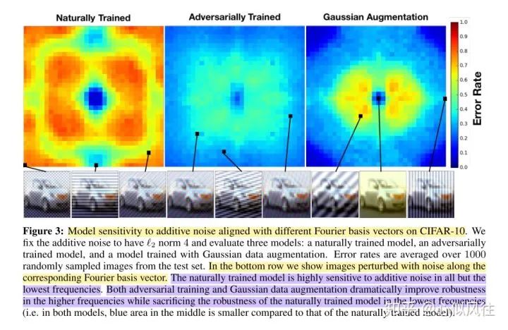
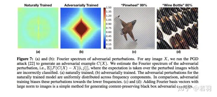 Image translation description: Model sensitivity to additive noise with different Fourier basis vectors on CIFAR-10. We fixed the additive noise to “L2 norm of 4” and evaluated three models: natural training model, adversarial training model, and Gaussian data augmentation training model. The average error rate was calculated for 1000 randomly sampled images from the test set. In the bottom row, we display images affected by noise along the corresponding Fourier basis vectors. The naturally trained model is highly sensitive to all additive noise except for the lowest frequencies. Both adversarial training and Gaussian data augmentation significantly improve robustness under high frequencies while sacrificing the robustness of the naturally trained model under low frequencies (i.e., in both models, the intermediate blue region is smaller than that of the naturally trained model).
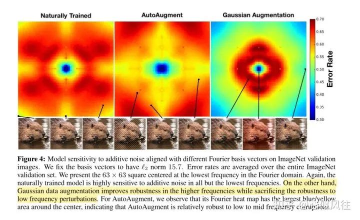
 Image translation description: Sensitivity of models to additive noise with different Fourier basis vectors on ImageNet validation images. We fixed the basis vector to an L2 norm value of 15.7. The error rate is the average error rate across the entire ImageNet validation set. A 63×63 square centered on the lowest frequency in the Fourier domain is provided. Similarly, the naturally trained model is highly sensitive to all additive noise except for the lowest frequencies. On the other hand, Gaussian data augmentation improves robustness under high frequencies while sacrificing robustness under low-frequency perturbations. For AutoAugment, we observe that its Fourier heatmap has the largest blue/yellow area around the center, indicating that AutoAugment is relatively robust against low-frequency to mid-frequency disturbances.
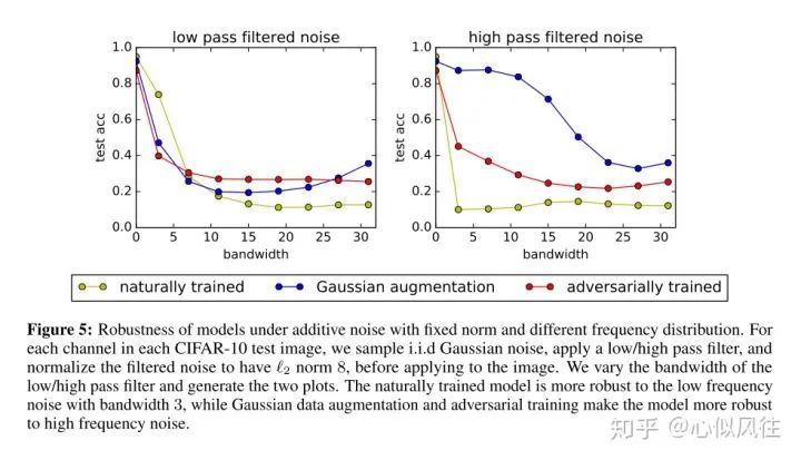
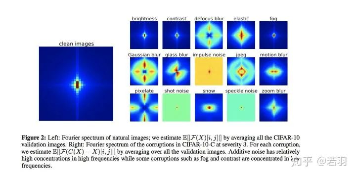 Image translation description: Robustness of models under additive noise with fixed norms and different frequency distributions. For each channel in each CIFAR-10 test image, we sample independent identically distributed Gaussian noise, apply low/high-pass filters, and normalize the filtered noise to an L2 norm value of 8 before applying it to the image. We vary the bandwidth of the low/high-pass filters to generate two curves. The naturally trained model shows stronger robustness against low-frequency noise with a bandwidth of 3, while Gaussian data augmentation and adversarial training enhance model robustness against high-frequency noise.
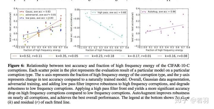 Image translation description: The relationship between the high-frequency energy fraction of CIFAR-10-C corrupted images and test accuracy. Each scatter point in the plot represents the evaluation results of a specific model against a specific corruption type. The x-axis represents the high-frequency energy score of the corruption type, while the y-axis represents the change in test accuracy compared to the naturally trained model. Overall, Gaussian data augmentation, adversarial training, and adding low-pass filters improve robustness against high-frequency corruption while reducing robustness against low-frequency corruption. Applying high-pass filters has a more significant accuracy drop for high-frequency corruption compared to low-frequency corruption. AutoAugment improves robustness against nearly all corruptions and achieves the best overall performance. The legend at the bottom shows the slope (K) and residual (r) of each fitted line.
 Image translation description: (a) and (b): Fourier spectrum of adversarial perturbations, given an image X, initiate PGD attacks to obtain adversarial samples C(X), estimating the Fourier spectrum of adversarial perturbations that cause misclassification of the image; (a) is the spectrum obtained from natural training; (b) is the spectrum obtained from adversarial training. The adversarial perturbations of the naturally trained model are uniformly distributed across frequency components. In contrast, adversarial training causes these perturbations to be biased toward lower frequencies. (C) and (D): Adding Fourier basis vectors with large norms to images is a simple method to generate content-preserving black-box adversarial examples.
1) Adversarial training focuses on some high-frequency components rather than solely fixating on low-frequency components.
2) AutoAugment helps improve robustness.
The open-source code mainly teaches how to draw diagrams similar to those in the paper.
Additionally, another paper from Eric Xing’s group, previously published on Zhihu’s self-media:
High-frequency Component Helps Explain the Generalization of Convolutional Neural Networks
https://arxiv.org/pdf/1905.13545.pdf
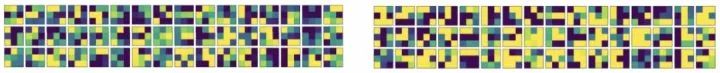
Visualization of convolution from natural training versus adversarial training
The paper experimented with several methods:
Image translation description: (a) and (b): Fourier spectrum of adversarial perturbations, given an image X, initiate PGD attacks to obtain adversarial samples C(X), estimating the Fourier spectrum of adversarial perturbations that cause misclassification of the image; (a) is the spectrum obtained from natural training; (b) is the spectrum obtained from adversarial training. The adversarial perturbations of the naturally trained model are uniformly distributed across frequency components. In contrast, adversarial training causes these perturbations to be biased toward lower frequencies. (C) and (D): Adding Fourier basis vectors with large norms to images is a simple method to generate content-preserving black-box adversarial examples.
1) Adversarial training focuses on some high-frequency components rather than solely fixating on low-frequency components.
2) AutoAugment helps improve robustness.
The open-source code mainly teaches how to draw diagrams similar to those in the paper.
Additionally, another paper from Eric Xing’s group, previously published on Zhihu’s self-media:
High-frequency Component Helps Explain the Generalization of Convolutional Neural Networks
https://arxiv.org/pdf/1905.13545.pdf
Visualization of convolution from natural training versus adversarial training
The paper experimented with several methods:
-
For a trained model, we adjusted its weights to make the convolution kernels smoother;
-
Directly filtering out high-frequency information from the trained convolution kernels;
-
Adding regularization during the training of convolutional neural networks to make the weights at adjacent positions closer.
Then the conclusion is drawn:
Focusing on low-frequency information helps improve generalization; high-frequency components may relate to adversarial attacks, but should not be too dogmatic.
The contribution is to provide detailed experiments demonstrating that Batch Normalization is useful for fitting high-frequency components and improving generalization.
Finally, it all comes down to mere talk.
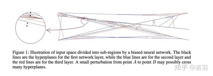
On this side, Professor Xu proves that the smoothness of ReLU aids function optimization; on the other side, a recent work called Bandlimiting Neural Networks Against Adversarial Attacks
https://arxiv.org/pdf/1905.12797.pdf
The ReLU function obtains a piecewise linear function
Can be decomposed into numerous frequency components.
For N=1000 nodes in the hidden layer and input dimension n=200, the maximum number of regions is approximately equal to 10^200. In other words, even a moderately sized neural network can partition the input space into a vast number of sub-regions, easily exceeding the total number of atoms in the universe. When we learn neural networks, we cannot expect at least one sample in each region. For those areas with no training samples, the results of linear functions can be arbitrary since they do not contribute to the training target function at all. Of course, most of these areas are very small. When we measure the expected loss function over the entire space, their contributions can be negligible, as the chance of random sampling points falling into these tiny regions is very small. However, adversarial attacks bring new challenges because adversarial samples are not naturally sampled. Considering the total number of regions is enormous, these tiny regions are almost everywhere in the input space. For any data point in the input space, we can almost certainly find such a tiny region where the linear function is arbitrary. If a point within this tiny region is chosen, the output of the neural network may be unexpected. These tiny regions are the fundamental reason why neural networks are vulnerable to adversarial attacks.
Then, a method for adversarial defense is proposed, which is unclear; the audience is welcome to read the paper and provide insights in the comment section.
Although there is procrastination, I will share other related and interesting papers when I see them.
https://www.zhihu.com/question/59532432/answer/1510340606
After receiving the invitation, I followed this question for a while, thinking that when someone with destiny answers this question, I can get the answer for free without spending time, secretly delighted. However, after waiting for a long time, no one gave a serious and detailed answer. So I can only come out and throw a brick to attract jade.
It’s amazing that I just read an article about understanding and analyzing model robustness from the frequency domain, and part of the content of this article also analyzes this issue, and very coincidentally: the experiments also used ResNet. Isn’t that a coincidence!
First, let me post the name of the paper:
A Fourier Perspective on Model Robustness in Computer Vision [1]
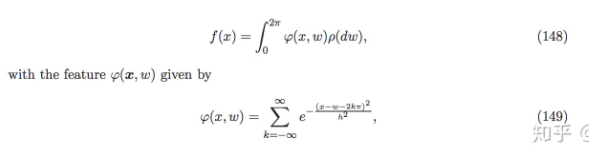
First of all, the deep learning model has achieved unprecedented success, but there is a significant problem: its robustness is poor, that is, when a little corruption is added to certain test images, the images will be misclassified. One method to enhance robustness is to perform data augmentation on the training set images, allowing the trained model to resist corruption. However, the author found that the same data augmentation methods, such as Gaussian augmentation and adversarial training, do not improve robustness for all corruption situations. The author raises a question: Why does the same augmentation method enhance performance for some corruption but reduce performance for others?
Then, the author proposes a hypothesis: Could it be that different corruptions provide different frequency information?
For CIFAR-10, the author used Wide ResNet-28-10;
For ImageNet, the author used ResNet-50.
The author analyzes the impact of different frequency information in images on the prediction accuracy of naturally trained models.
As shown in the figure above, the author conducted experiments using the ResNet-50 model trained on ImageNet.
For low-frequency information, the author directly applied a low-pass filter in the frequency domain of the test images, allowing different amounts of low-frequency signals to pass through with varying filter sizes; four typical filtered images are shown at the top of the chart.
For high-frequency information, the author applied a high-pass filter in the frequency domain of the images and performed normalization. Different filter sizes allowed varying amounts of high-frequency signals to pass through; four typical filtered images are shown on the right side of the chart.
The x-axis of the chart represents the size of the filter, while the y-axis represents classification accuracy.
The charts above demonstrate that even with a very small low-pass filter size, the image appears as a color block, and the human eye cannot distinguish what it is, yet the model still achieves over 30% accuracy (the first image derived from the low-pass filter). For the high-pass filtered portion (the second image from the top), even when the human eye cannot discern what is in the image, the model still achieves 50% accuracy. Moreover, when low-frequency information is scarce, increasing low-frequency information can rapidly enhance accuracy, but after reaching a certain amount, it no longer has an effect; the impact of high-frequency information on accuracy gradually increases and is not as rapid as that of low-frequency information.
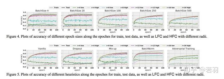
For the CIFAR-10 training set, the author analyzes the sensitivity of the Wide ResNet-28-10 model to additive noise.
The center of the image is the low-frequency signal area, with increasing frequency towards the edges.
The training set is CIFAR-10, and the trained model is Wide ResNet-28-10.
The naturally trained model is highly sensitive to all frequencies except for low-frequency corruption noise, while adversarial training and Gaussian augmentation improve the model’s robustness against high-frequency corruption (lower error rate).
For the ImageNet training set, the author analyzes the sensitivity of the ResNet-50 model to additive noise.
The naturally trained model is highly sensitive to all frequencies except for low-frequency corruption noise; Gaussian augmentation sacrifices robustness against low-frequency perturbations but improves it against high-frequency ones. For AutoAugment, robustness gradually decreases for low, mid, and high frequencies.
The impact of high-frequency and low-frequency signals on test accuracy as bandwidth increases.
The training set is CIFAR-10, and the model is Wide ResNet-28-10.
Compared to the naturally trained model, as the bandwidth of the noise filter increases, test accuracy decreases, while we find that the accuracy of the models derived from Gaussian augmentation and adversarial training is higher than that of the naturally trained model.
Supplement 1:According to the answer from @Lost under this question, I also recommend everyone to check out the paper he mentioned Frequency Principle: Fourier Analysis Sheds Light on Deep Neural Networks[2]
https://arxiv.org/pdf/1901.06523.pdf
Supplement 2:I also recommend everyone to read the following paper High-frequency Component Helps Explain the Generalization of Convolutional Neural Network[3]
https://openaccess.thecvf.com/content_CVPR_2020/papers/Wang_High-Frequency_Component_Helps_Explain_the_Generalization_of_Convolutional_Networks_CVPR_2020_paper.pdf
[1] A Fourier Perspective on Model Robustness in Computer Vision
[2] Frequency Principle: Fourier Analysis Sheds Light on Deep Neural Networks
[3] High-frequency Component Helps Explain the Generalization of Convolutional Neural Network
https://www.zhihu.com/question/59532432/answer/1447173834
Recommended Reading
-
Understanding Different Types of Convolutional Layers in Neural Networks
-
Overview of Few-shot Segmentation Algorithms Based on Deep Convolutional Neural Networks
-
Understanding the Self-attention Mechanism in Convolutional Neural Networks
ACCV 2020 International Fine-grained Network Image Recognition Competition Officially Launched!