Evolution of CNN Architectures: From LeNet to DenseNet

Editor | Fish Da

Reprinted from | Champion’s Trial Blog

Total words:21041 Images:18

Estimated reading time: 53 minutes

Convolutional Neural Networks (CNNs) have become a prominent framework in the field of deep learning, especially excelling in computer vision. Starting from LeNet in the 1990s, CNNs went through a decade of silence until AlexNet revived them in 2012. From ZF Net to VGG, GoogLeNet, ResNet, and the recent DenseNet, the networks have become deeper, with increasingly complex architectures and more sophisticated methods to solve the vanishing gradient problem during backpropagation. With the New Year holidays, let’s summarize the various classic architectures of CNNs and appreciate the beauty of the intellectual collision among the great minds in the evolution of CNNs.

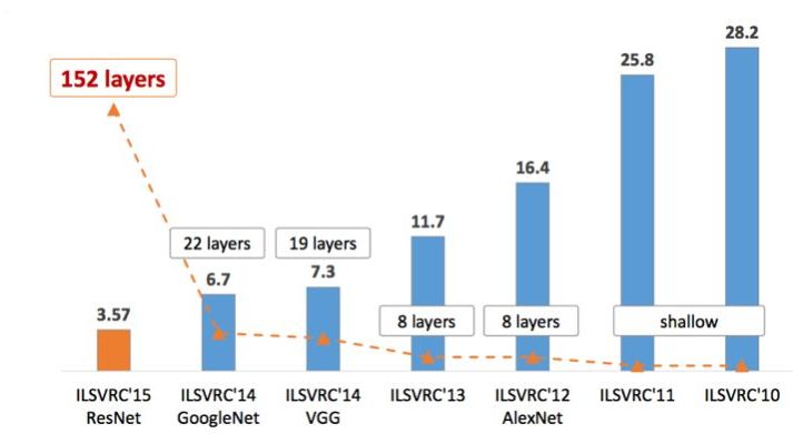
The above image shows the Top-5 error rates of ILSVRC over the years. We will introduce the classic networks in the order of their appearance.

This article will discuss the following classic convolutional neural networks:

LeNet
AlexNet
ZF
VGG
GoogLeNet
ResNet
DenseNet

Foundational Work: LeNet

Highlights: Defined the basic components of CNNs, the ancestor of CNNs.

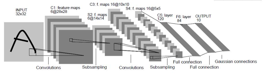
LeNet was proposed by LeCun, the father of convolutional neural networks, in 1998 to solve visual tasks for handwritten digit recognition. Since then, the fundamental architecture of CNNs has been established: convolutional layers, pooling layers, and fully connected layers. The LeNet used in various deep learning frameworks today is a simplified and improved version of LeNet-5 (the -5 indicates it has 5 layers), which differs slightly from the original LeNet, such as changing the activation function to the now widely used ReLU.

LeNet-5 differs from the existing conv->pool->ReLU routine; it uses the approach of conv1->pool->conv2->pool2 followed by a fully connected layer, but the pattern of having a pooling layer immediately after a convolutional layer remains unchanged.

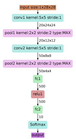
Taking the classic LeNet-5 as an example, let’s analyze it in depth:

First, the input image is a single-channel image of size 28*28, represented as a matrix [1,28,28].
The size of the convolution kernel used in the first convolutional layer (conv1) is 5*5, with a stride of 1, and the number of convolution kernels is 20. After this layer, the image size becomes 24, calculated as 28-5+1=24, resulting in an output matrix of [20,24,24].
The first pooling layer (pool) has a kernel size of 2*2 and a stride of 2, which is non-overlapping max pooling. After pooling, the image size is halved to 12×12, resulting in an output matrix of [20,12,12].
The second convolutional layer (conv2) has a kernel size of 5*5, a stride of 1, and the number of convolution kernels is 50. After convolution, the image size becomes 8, calculated as 12-5+1=8, resulting in an output matrix of [50,8,8].
The second pooling layer (pool2) has a kernel size of 2*2 and a stride of 2, which is non-overlapping max pooling. After pooling, the image size is halved to 4×4, resulting in an output matrix of [50,4,4].
After pool2, a fully connected layer (fc1) is added with 500 neurons, followed by a ReLU activation function.
Then another fully connected layer (fc2) is added with 10 neurons, producing a 10-dimensional feature vector for training classification into 10 digits, which is fed into a softmax classifier to obtain the probability output of the classification result.

LeNet implemented in Keras:

def LeNet():
    model = Sequential()
    model.add(Conv2D(32,(5,5),strides=(1,1),input_shape=(28,28,1),padding='valid',activation='relu',kernel_initializer='uniform'))
    model.add(MaxPooling2D(pool_size=(2,2)))
    model.add(Conv2D(64,(5,5),strides=(1,1),padding='valid',activation='relu',kernel_initializer='uniform'))
    model.add(MaxPooling2D(pool_size=(2,2)))
    model.add(Flatten())
    model.add(Dense(100,activation='relu'))
    model.add(Dense(10,activation='softmax'))
    return model

The Return of the King: AlexNet

AlexNet won the ImageNet competition in 2012 with an absolute advantage of 10.9 percentage points over the second place, marking the rise of deep learning and convolutional neural networks. The emergence of AlexNet can be seen as the return of the king of convolutional neural networks.

Highlights:

Deeper networks
Data augmentation
ReLU
Dropout
Local Response Normalization (LRN)

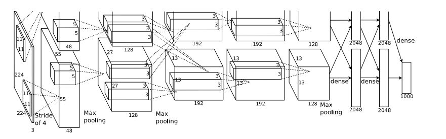
Taking the architecture of AlexNet as an example, this network has 5 convolutional layers followed by three fully connected layers, with the final softmax output classifying into 1000 categories, focusing on the first two layers for detailed explanation.

AlexNet consists of 5 convolutional layers and three fully connected layers, which is significantly more than LeNet, but the overall process of the convolutional neural network remains unchanged, with just a deeper structure.
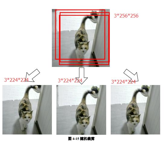
AlexNet addresses a classification problem with 1000 categories, with input images specified as 256×256 three-channel color images. To enhance the model’s generalization ability and avoid overfitting, the author used the strategy of random cropping to obtain images sized 3×224×224 from the original 256×256 images for network training.

Due to the use of multiple GPUs for training, the first convolutional layer has two identical branches to speed up training.
Analyzing one branch: The first convolutional layer (conv1) has a kernel size of 11×11, a stride of 4, and the number of convolution kernels is 48. The output matrix after convolution is [48,55,55]. The number 55 is somewhat confusing, and the author did not explain it. If calculated normally, (224-11)/4+1 != 55, indicating that padding was applied before convolution, padding the image to 227×227 first, then convolving (227-11)/4+1 = 55. The pixels processed by the relu1 unit generate the activated pixel layer, resulting in two groups of 48×55×55 pixel layer data. After max pooling with a scale of 3×3 and a stride of 2, the output matrix size becomes [48,27,27].

Training techniques used in AlexNet:

Data augmentation techniques to increase the model’s generalization ability.
Using ReLU instead of Sigmoid to speed up the convergence of SGD.
Dropout: The principle of dropout is similar to the ensemble method in shallow learning algorithms, where some neurons in the fully connected layers (dropout is introduced in the first two fully connected layers) are randomly deactivated with a certain probability (e.g., 0.5). Deactivated neurons do not participate in forward and backward propagation, effectively making about half of the neurons inactive. During testing, all neurons’ outputs are multiplied by 0.5. The introduction of dropout effectively alleviates overfitting.
Local Response Normalization (LRN): The basic idea of LRN is to select a location from a feature map and normalize the responses across the channels for that location. The motivation for local response normalization is that we might not need too many highly activated neurons for each position in the feature map. However, many researchers later found LRN to be less effective, as it is not crucial, and it is not used in training networks today.

AlexNet implemented in Keras:

def AlexNet():
    model = Sequential()
    model.add(Conv2D(96,(11,11),strides=(4,4),input_shape=(227,227,3),padding='valid',activation='relu',kernel_initializer='uniform'))
    model.add(MaxPooling2D(pool_size=(3,3),strides=(2,2)))
    model.add(Conv2D(256,(5,5),strides=(1,1),padding='same',activation='relu',kernel_initializer='uniform'))
    model.add(MaxPooling2D(pool_size=(3,3),strides=(2,2)))
    model.add(Conv2D(384,(3,3),strides=(1,1),padding='same',activation='relu',kernel_initializer='uniform'))
    model.add(Conv2D(384,(3,3),strides=(1,1),padding='same',activation='relu',kernel_initializer='uniform'))
    model.add(Conv2D(256,(3,3),strides=(1,1),padding='same',activation='relu',kernel_initializer='uniform'))
    model.add(MaxPooling2D(pool_size=(3,3),strides=(2,2)))
    model.add(Flatten())
    model.add(Dense(4096,activation='relu'))
    model.add(Dropout(0.5))
    model.add(Dense(4096,activation='relu'))
    model.add(Dropout(0.5))
    model.add(Dense(1000,activation='softmax'))
    return model

Steady Progress: ZF-Net

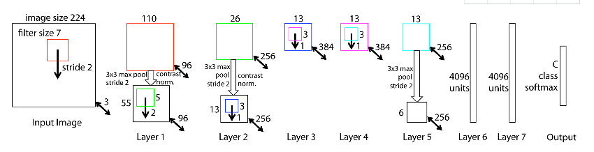
ZFNet won the ImageNet classification task in 2013. Its network structure did not change much, only some parameters were adjusted, leading to a significant performance improvement over AlexNet. ZF-Net simply changed the kernel size of the first convolutional layer from 11 to 7, the stride from 4 to 2, and the third, fourth, and fifth convolutional layers to 384, 384, and 256 respectively. This year’s ImageNet was relatively calm, and the champion ZF-Net did not have the same classic network architecture reputation as in previous years.

ZF-Net implemented in Keras:

def ZF_Net():
    model = Sequential()  
    model.add(Conv2D(96,(7,7),strides=(2,2),input_shape=(224,224,3),padding='valid',activation='relu',kernel_initializer='uniform'))  
    model.add(MaxPooling2D(pool_size=(3,3),strides=(2,2)))  
    model.add(Conv2D(256,(5,5),strides=(2,2),padding='same',activation='relu',kernel_initializer='uniform'))  
    model.add(MaxPooling2D(pool_size=(3,3),strides=(2,2)))  
    model.add(Conv2D(384,(3,3),strides=(1,1),padding='same',activation='relu',kernel_initializer='uniform'))  
    model.add(Conv2D(384,(3,3),strides=(1,1),padding='same',activation='relu',kernel_initializer='uniform'))  
    model.add(Conv2D(256,(3,3),strides=(1,1),padding='same',activation='relu',kernel_initializer='uniform'))  
    model.add(MaxPooling2D(pool_size=(3,3),strides=(2,2)))  
    model.add(Flatten())  
    model.add(Dense(4096,activation='relu'))  
    model.add(Dropout(0.5))  
    model.add(Dense(4096,activation='relu'))  
    model.add(Dropout(0.5))  
    model.add(Dense(1000,activation='softmax'))  
    return model

Going Deeper: VGG-Nets

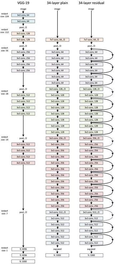
VGG-Nets, proposed by the Visual Geometry Group (VGG) at Oxford University, ranked first in the localization task and second in the classification task at the 2014 ImageNet competition. VGG can be seen as a deeper version of AlexNet. Both consist of convolutional layers and fully connected layers, and at that time, it was considered a very deep network with over ten layers, as indicated by its paper title (“Very Deep Convolutional Networks for Large-Scale Visual Recognition”). Of course, from today’s perspective, VGG can hardly be called a very deep network.

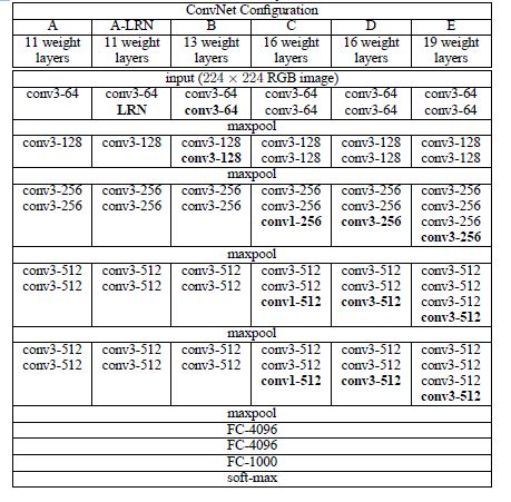
The table above describes the structure and birth process of VGG-Net. To address initialization (weight initialization) issues, VGG adopted a pre-training approach, commonly seen in classic neural networks, where a small network is trained first, and once stabilized, the network is gradually deepened. Table 1 reflects this process from left to right, and when the network is in stage D, the performance is optimal; hence the network in stage D is VGG-16! The network obtained in stage E is VGG-19! The 16 in VGG-16 indicates that the total number of layers (conv + fc) is 16, excluding the max pooling layers!

The following image shows the structure of VGG-16.

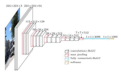
From the above image, it is evident that the structure of VGG-16 is very neat and significantly deeper than AlexNet. It contains multiple conv->conv->max_pool structures. The convolutional layers in VGG are all same convolutions, meaning the output image size after convolution is the same as the input size, and downsampling is achieved entirely through max pooling.

VGG’s attention lies in using smaller filter sizes and systematic convolution-pooling operations.

Highlights:

Convolutional layers use smaller filter sizes and intervals.

Compared to AlexNet, it can be seen that VGG-Nets use much smaller convolution kernels. For example, the first convolutional layer in AlexNet uses an 11×11 kernel, which is quite large. In contrast, VGG-Nets primarily use 1×1 and 3×3 small convolution kernels, which can replace larger filter sizes.

Advantages of the 3×3 convolution kernel:

Multiple 3×3 convolutional layers provide more non-linearity than a single large filter convolutional layer, making the decision function more decisive.
Multiple 3×3 convolutional layers have fewer parameters than a single large filter convolutional layer. Assuming the input and output feature map sizes are the same (C), the number of parameters for three 3×3 convolutional layers is 3×(3×3×C×C)=27CC; for a single 7×7 convolutional layer, the number of parameters is 49CC; thus, three 3×3 filters can be seen as a decomposition of a 7×7 filter (with non-linear decompositions in the intermediate layer).

Advantages of the 1×1 convolution kernel:

It performs linear transformations on the input without affecting the input-output dimensions, followed by ReLU for non-linear processing, enhancing the network’s non-linear expressiveness.

VGG-16 implemented in Keras:

def VGG_16():   
    model = Sequential()
    
    model.add(Conv2D(64,(3,3),strides=(1,1),input_shape=(224,224,3),padding='same',activation='relu',kernel_initializer='uniform'))
    model.add(Conv2D(64,(3,3),strides=(1,1),padding='same',activation='relu',kernel_initializer='uniform'))
    model.add(MaxPooling2D(pool_size=(2,2)))
    
    model.add(Conv2D(128,(3,2),strides=(1,1),padding='same',activation='relu',kernel_initializer='uniform'))
    model.add(Conv2D(128,(3,3),strides=(1,1),padding='same',activation='relu',kernel_initializer='uniform'))
    model.add(MaxPooling2D(pool_size=(2,2)))
    
    model.add(Conv2D(256,(3,3),strides=(1,1),padding='same',activation='relu',kernel_initializer='uniform'))
    model.add(Conv2D(256,(3,3),strides=(1,1),padding='same',activation='relu',kernel_initializer='uniform'))
    model.add(Conv2D(256,(3,3),strides=(1,1),padding='same',activation='relu',kernel_initializer='uniform'))
    model.add(MaxPooling2D(pool_size=(2,2)))
    
    model.add(Conv2D(512,(3,3),strides=(1,1),padding='same',activation='relu',kernel_initializer='uniform'))
    model.add(Conv2D(512,(3,3),strides=(1,1),padding='same',activation='relu',kernel_initializer='uniform'))
    model.add(Conv2D(512,(3,3),strides=(1,1),padding='same',activation='relu',kernel_initializer='uniform'))
    model.add(MaxPooling2D(pool_size=(2,2)))
    
    model.add(Conv2D(512,(3,3),strides=(1,1),padding='same',activation='relu',kernel_initializer='uniform'))
    model.add(Conv2D(512,(3,3),strides=(1,1),padding='same',activation='relu',kernel_initializer='uniform'))
    model.add(Conv2D(512,(3,3),strides=(1,1),padding='same',activation='relu',kernel_initializer='uniform'))
    model.add(MaxPooling2D(pool_size=(2,2)))
    
    model.add(Flatten())
    model.add(Dense(4096,activation='relu'))
    model.add(Dropout(0.5))
    model.add(Dense(4096,activation='relu'))
    model.add(Dropout(0.5))
    model.add(Dense(1000,activation='softmax'))
    
    return model

Driving Force: GoogLeNet

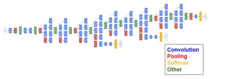
GoogLeNet won the championship in the 2014 ImageNet classification task, defeating VGG-Nets. Its strength is undoubtedly profound. Unlike AlexNet and VGG-Nets, which purely rely on deepening the network structure to improve performance, GoogLeNet innovatively introduced the Inception structure while deepening the network (22 layers), further advancing the study of convolutional neural networks.

Highlights:

Introduction of the Inception structure
Auxiliary loss units in intermediate layers
All subsequent fully connected layers replaced with simple global average pooling

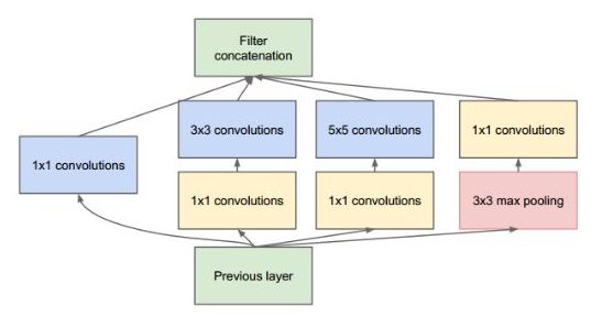
The structure in the image above illustrates Inception, where the convolution strides are all 1, and to maintain the size of the feature response maps, zero padding is used. Each convolution layer is immediately followed by a ReLU layer. Before the output, there is a layer called concatenate, meaning to “stack” the four groups of different types but same-sized feature response maps side by side, forming new feature response maps. The Inception structure mainly does two things: 1. Extracts features from the input feature response maps using three different scales of convolution kernels (1×1, 3×3, and 5×5) and pooling, and 2. Reduces computational load while allowing information to be transmitted through fewer connections to achieve sparser characteristics, using 1×1 convolution kernels for dimensionality reduction.

Let’s discuss the role of the 1×1 convolution kernel in detail and how it achieves dimensionality reduction. The calculations are as follows: for a single-channel input, a 1×1 convolution does not achieve dimensionality reduction, but for multi-channel inputs, it does. Suppose you have 256 feature inputs and 256 feature outputs, and the Inception layer only executes 3×3 convolutions. This means a total of 256×256×3×3 convolutions (589000 multiplication-accumulation operations). This may exceed our computational budget, for example, taking 0.5 milliseconds to run this layer on Google servers. As an alternative, we decide to reduce the number of features to convolve, say down to 64 (256/4). In this case, we first perform a 1×1 convolution from 256 to 64, then perform 64 convolutions on all Inception branches, and finally apply a 1×1 convolution from 64 back to 256.

256×64×1×1 = 16000
64×64×3×3 = 36000
64×256×1×1 = 16000

The current computational load is approximately 70000 (i.e., 16000+36000+16000), compared to the previous approximately 600000, which is nearly a tenfold reduction. This achieves dimensionality reduction through smaller convolution kernels.

Now, consider another question: why must we use 1×1 convolution kernels? Can’t 3×3 also work? Consider a matrix input of [50,200,200]. We can use 20 1×1 convolution kernels to convolve, obtaining an output of [20,200,200]. One might ask, can’t I also achieve a [20,200,200] matrix output with 20 3×3 convolution kernels? Why use 1×1 convolution kernels? Let’s calculate the convolution parameters to find out. For 1×1, the total number of parameters is: 20×200×200×(1×1); for 3×3, the total number of parameters is: 20×200×200×(3×3). We can see that the total number of parameters for 1×1 is only one-ninth that of 3×3!

In the GoogLeNet network structure, there are three loss units, designed to assist the network’s convergence. By adding auxiliary loss units in the intermediate layers, the aim is to ensure that low-level features have good discriminative ability during loss calculation, thus allowing the network to be better trained. In the paper, the calculations of these two auxiliary loss units are multiplied by 0.3 and added to the final loss as the overall loss function for training the network.

Another highlight of GoogLeNet is that all subsequent fully connected layers are replaced with simple global average pooling, resulting in fewer parameters. In AlexNet, the last three fully connected layers account for about 90% of the total parameters. With a large network, the width and depth allow GoogLeNet to remove fully connected layers without affecting accuracy, achieving 93.3% accuracy on ImageNet, and even faster than VGG.

GoogLeNet implemented in Keras:

def Conv2d_BN(x, nb_filter,kernel_size, padding='same',strides=(1,1),name=None):
    if name is not None:
        bn_name = name + '_bn'
        conv_name = name + '_conv'
    else:
        bn_name = None
        conv_name = None

    x = Conv2D(nb_filter,kernel_size,padding=padding,strides=strides,activation='relu',name=conv_name)(x)
    x = BatchNormalization(axis=3,name=bn_name)(x)
    return x

def Inception(x,nb_filter):
    branch1x1 = Conv2d_BN(x,nb_filter,(1,1), padding='same',strides=(1,1),name=None)

    branch3x3 = Conv2d_BN(x,nb_filter,(1,1), padding='same',strides=(1,1),name=None)
    branch3x3 = Conv2d_BN(branch3x3,nb_filter,(3,3), padding='same',strides=(1,1),name=None)

    branch5x5 = Conv2d_BN(x,nb_filter,(1,1), padding='same',strides=(1,1),name=None)
    branch5x5 = Conv2d_BN(branch5x5,nb_filter,(1,1), padding='same',strides=(1,1),name=None)

    branchpool = MaxPooling2D(pool_size=(3,3),strides=(1,1),padding='same')(x)
    branchpool = Conv2d_BN(branchpool,nb_filter,(1,1),padding='same',strides=(1,1),name=None)

    x = concatenate([branch1x1,branch3x3,branch5x5,branchpool],axis=3)

    return x

def GoogLeNet():
    inpt = Input(shape=(224,224,3))
    #padding = 'same'，填充为(步长-1）/2,还可以用ZeroPadding2D((3,3))
    x = Conv2d_BN(inpt,64,(7,7),strides=(2,2),padding='same')
    x = MaxPooling2D(pool_size=(3,3),strides=(2,2),padding='same')(x)
    x = Conv2d_BN(x,192,(3,3),strides=(1,1),padding='same')
    x = MaxPooling2D(pool_size=(3,3),strides=(2,2),padding='same')(x)
    x = Inception(x,64)#256
    x = Inception(x,120)#480
    x = MaxPooling2D(pool_size=(3,3),strides=(2,2),padding='same')(x)
    x = Inception(x,128)#512
    x = Inception(x,128)
    x = Inception(x,128)
    x = Inception(x,132)#528
    x = Inception(x,208)#832
    x = MaxPooling2D(pool_size=(3,3),strides=(2,2),padding='same')(x)
    x = Inception(x,208)
    x = Inception(x,256)#1024
    x = AveragePooling2D(pool_size=(7,7),strides=(7,7),padding='same')(x)
    x = Dropout(0.4)(x)
    x = Dense(1000,activation='relu')(x)
    x = Dense(1000,activation='softmax')(x)
    model = Model(inpt,x,name='inception')
    return model

Milestone Innovation: ResNet

In 2015, Kaiming He introduced ResNet, which swept all competitors in ISLVRC and COCO, winning the championship. ResNet made significant innovations in network structure, no longer simply stacking layers. ResNet represents a new approach in convolutional neural networks and is a milestone event in the development of deep learning.

Highlights:

Very deep, exceeding hundreds of layers
Introduces residual units to solve the degradation problem

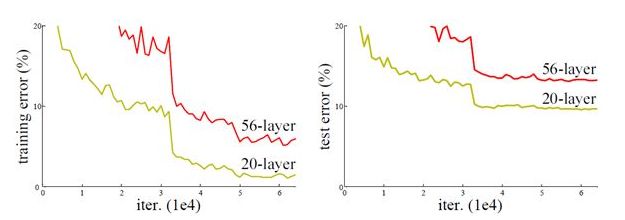
As seen earlier, with the increase in network depth, the accuracy should also increase. However, care must be taken to avoid overfitting. One problem with increasing network depth is that the added layers may have small gradient signals for parameter updates because gradients are propagated from back to front. With deeper networks, the gradients for earlier layers become very small, meaning they essentially stop learning, leading to the vanishing gradient problem. A second issue with training deeper networks is that it implies a larger parameter space, making optimization more challenging. Therefore, simply increasing the depth can lead to higher training errors; deep networks may converge but start to degrade, leading to greater errors, as illustrated in the figure below, where a 56-layer network performs worse than a 20-layer network, not due to overfitting (the training error remains high) but because of the degradation problem. ResNet designs a residual module that allows us to train deeper networks.

To understand the essence of ResNet, let’s analyze the residual unit in detail.

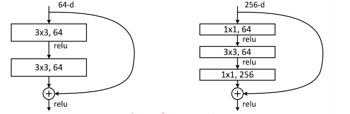
From the diagram below, data follows two paths: one is the conventional path, and the other is a shortcut that directly implements an identity mapping. This structure with a shortcut connection can effectively address the degradation problem. If we consider the input-output relationship of a module in the network as y=H(x), the optimization target for the variable part is no longer H(x). If we denote the part to be optimized as F(x), then H(x)=F(x)+x, meaning F(x)=H(x)-x. In the assumption of identity mapping, y=x represents the observed value, so F(x) corresponds to the residual, hence the name residual network. The reason for this design is that learning the residual F(X) is simpler than directly learning H(X). The idea is to learn the difference between input and output, making the absolute quantity a relative quantity (H(x)-x represents how much the output changes relative to the input), simplifying the optimization process.

Considering that the dimensions of x and F(X) may not match, dimensionality matching is required. The paper proposes two methods to address this issue (three methods were actually proposed, but the third significantly degraded performance and was therefore not adopted):

Zero padding: Padding the identity layer with zeros to complete the dimensions. This method does not add extra parameters.
Projection: Using a 1×1 convolution kernel on the identity layer to increase dimensions. This method adds extra parameters.

The following diagram shows two forms of residual modules: the left is the conventional residual module consisting of two 3×3 convolution kernels, but as the network deepens, this structure may not be very effective in practice. To address this issue, the right diagram illustrates the “bottleneck residual module,” which is composed of 1×1, 3×3, and 1×1 convolution layers, where the 1×1 convolution can serve to increase or decrease dimensions, allowing the 3×3 convolution to operate on relatively lower-dimensional inputs, thereby improving computational efficiency.

ResNet-50 implemented in Keras:

def Conv2d_BN(x, nb_filter,kernel_size, strides=(1,1), padding='same',name=None):
    if name is not None:
        bn_name = name + '_bn'
        conv_name = name + '_conv'
    else:
        bn_name = None
        conv_name = None

    x = Conv2D(nb_filter,kernel_size,padding=padding,strides=strides,activation='relu',name=conv_name)(x)
    x = BatchNormalization(axis=3,name=bn_name)(x)
    return x

def Conv_Block(inpt,nb_filter,kernel_size,strides=(1,1), with_conv_shortcut=False):
    x = Conv2d_BN(inpt,nb_filter=nb_filter[0],kernel_size=(1,1),strides=strides,padding='same')
    x = Conv2d_BN(x, nb_filter=nb_filter[1], kernel_size=(3,3), padding='same')
    x = Conv2d_BN(x, nb_filter=nb_filter[2], kernel_size=(1,1), padding='same')
    if with_conv_shortcut:
        shortcut = Conv2d_BN(inpt,nb_filter=nb_filter[2],strides=strides,kernel_size=kernel_size)
        x = add([x,shortcut])
        return x
    else:
        x = add([x,inpt])
        return x

def ResNet50():
    inpt = Input(shape=(224,224,3))
    x = ZeroPadding2D((3,3))(inpt)
    x = Conv2d_BN(x,nb_filter=64,kernel_size=(7,7),strides=(2,2),padding='valid')
    x = MaxPooling2D(pool_size=(3,3),strides=(2,2),padding='same')(x)
    
    x = Conv_Block(x,nb_filter=[64,64,256],kernel_size=(3,3),strides=(1,1),with_conv_shortcut=True)
    x = Conv_Block(x,nb_filter=[64,64,256],kernel_size=(3,3))
    x = Conv_Block(x,nb_filter=[64,64,256],kernel_size=(3,3))
    
    x = Conv_Block(x,nb_filter=[128,128,512],kernel_size=(3,3),strides=(2,2),with_conv_shortcut=True)
    x = Conv_Block(x,nb_filter=[128,128,512],kernel_size=(3,3))
    x = Conv_Block(x,nb_filter=[128,128,512],kernel_size=(3,3))
    x = Conv_Block(x,nb_filter=[128,128,512],kernel_size=(3,3))
    
    x = Conv_Block(x,nb_filter=[256,256,1024],kernel_size=(3,3),strides=(2,2),with_conv_shortcut=True)
    x = Conv_Block(x,nb_filter=[256,256,1024],kernel_size=(3,3))
    x = Conv_Block(x,nb_filter=[256,256,1024],kernel_size=(3,3))
    x = Conv_Block(x,nb_filter=[256,256,1024],kernel_size=(3,3))
    x = Conv_Block(x,nb_filter=[256,256,1024],kernel_size=(3,3))
    x = Conv_Block(x,nb_filter=[256,256,1024],kernel_size=(3,3))
    
    x = Conv_Block(x,nb_filter=[512,512,2048],kernel_size=(3,3),strides=(2,2),with_conv_shortcut=True)
    x = Conv_Block(x,nb_filter=[512,512,2048],kernel_size=(3,3))
    x = Conv_Block(x,nb_filter=[512,512,2048],kernel_size=(3,3))
    x = AveragePooling2D(pool_size=(7,7))(x)
    x = Flatten()(x)
    x = Dense(1000,activation='softmax')(x)
    
    model = Model(inputs=inpt,outputs=x)
    return model

Continuing the Legacy: DenseNet

Since the introduction of ResNet, various variants of ResNet have emerged, each with its own characteristics and improvements in network performance. The final network introduced in this article is DenseNet, awarded the best paper at CVPR 2017. DenseNet (Dense Convolutional Network) primarily compares itself with ResNet and Inception networks, borrowing ideas yet presenting a completely new structure. The network structure is not complex but highly effective, surpassing ResNet across CIFAR metrics. DenseNet can be said to have absorbed the essence of ResNet while making more innovative contributions, further enhancing network performance.

Highlights:

Dense connections: alleviate the vanishing gradient problem, strengthen feature propagation, encourage feature reuse, and significantly reduce the parameter count.

DenseNet is a convolutional neural network with dense connections. In this network, there are direct connections between any two layers, meaning the input of each layer is the union of the outputs from all previous layers, and the feature maps learned by that layer are directly passed to all subsequent layers as input. The diagram below illustrates a dense block of DenseNet, where the structure is similar to the bottleneck in ResNet: BN-ReLU-Conv(1×1)-BN-ReLU-Conv(3×3). A DenseNet consists of multiple such blocks. Each DenseBlock is separated by transition layers composed of BN->Conv(1×1)−>averagePooling(2×2).

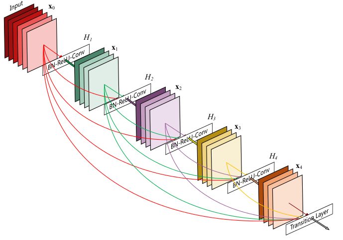
Do dense connections lead to redundancy? No! The term dense connections might imply a significant increase in network parameters and computation. However, DenseNet is more efficient than other networks due to the reduced computational load for each layer and the reuse of features. DenseNet allows the input from layer l to directly influence all subsequent layers, with its output being: xl=Hl([X0,X1,…,xl−1]), where [x0,x1,…,xl−1] merges the previous feature maps along the channel dimension. Since each layer contains information from all previous layers, it only requires a small number of feature maps, which is why DenseNet’s parameter count is significantly lower than other models. This dense connectivity effectively reduces the vanishing gradient phenomenon, making deeper networks manageable.

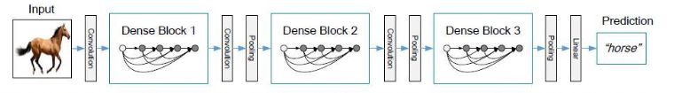
It should be noted that dense connectivity occurs only within a dense block; there is no dense connectivity between different dense blocks, as illustrated in the diagram below.

There’s no such thing as a free lunch; networks are no exception. Achieving better convergence rates at the same layer depth comes with an additional cost, one of which is significant memory usage.

DenseNet-121 implemented in Keras:

def DenseNet121(nb_dense_block=4, growth_rate=32, nb_filter=64, reduction=0.0, dropout_rate=0.0, weight_decay=1e-4, classes=1000, weights_path=None):
    '''Instantiate the DenseNet 121 architecture,
        # Arguments
            nb_dense_block: number of dense blocks to add to end
            growth_rate: number of filters to add per dense block
            nb_filter: initial number of filters
            reduction: reduction factor of transition blocks.
            dropout_rate: dropout rate
            weight_decay: weight decay factor
            classes: optional number of classes to classify images
            weights_path: path to pre-trained weights
        # Returns
            A Keras model instance.
    '''
    eps = 1.1e-5

    # compute compression factor
    compression = 1.0 - reduction

    # Handle Dimension Ordering for different backends
    global concat_axis
    if K.image_dim_ordering() == 'tf':
      concat_axis = 3
      img_input = Input(shape=(224, 224, 3), name='data')
    else:
      concat_axis = 1
      img_input = Input(shape=(3, 224, 224), name='data')

    # From architecture for ImageNet (Table 1 in the paper)
    nb_filter = 64
    nb_layers = [6,12,24,16] # For DenseNet-121

    # Initial convolution
    x = ZeroPadding2D((3, 3), name='conv1_zeropadding')(img_input)
    x = Convolution2D(nb_filter, 7, 7, subsample=(2, 2), name='conv1', bias=False)(x)
    x = BatchNormalization(epsilon=eps, axis=concat_axis, name='conv1_bn')(x)
    x = Scale(axis=concat_axis, name='conv1_scale')(x)
    x = Activation('relu', name='relu1')(x)
    x = ZeroPadding2D((1, 1), name='pool1_zeropadding')(x)
    x = MaxPooling2D((3, 3), strides=(2, 2), name='pool1')(x)

    # Add dense blocks
    for block_idx in range(nb_dense_block - 1):
        stage = block_idx+2
        x, nb_filter = dense_block(x, stage, nb_layers[block_idx], nb_filter, growth_rate, dropout_rate=dropout_rate, weight_decay=weight_decay)

        # Add transition_block
        x = transition_block(x, stage, nb_filter, compression=compression, dropout_rate=dropout_rate, weight_decay=weight_decay)
        nb_filter = int(nb_filter * compression)

    final_stage = stage + 1
    x, nb_filter = dense_block(x, final_stage, nb_layers[-1], nb_filter, growth_rate, dropout_rate=dropout_rate, weight_decay=weight_decay)

    x = BatchNormalization(epsilon=eps, axis=concat_axis, name='conv'+str(final_stage)+'_blk_bn')(x)
    x = Scale(axis=concat_axis, name='conv'+str(final_stage)+'_blk_scale')(x)
    x = Activation('relu', name='relu'+str(final_stage)+'_blk')(x)
    x = GlobalAveragePooling2D(name='pool'+str(final_stage))(x)

    x = Dense(classes, name='fc6')(x)
    x = Activation('softmax', name='prob')(x)

    model = Model(img_input, x, name='densenet')

    if weights_path is not None:
      model.load_weights(weights_path)

    return model

def conv_block(x, stage, branch, nb_filter, dropout_rate=None, weight_decay=1e-4):
    '''Apply BatchNorm, Relu, bottleneck 1x1 Conv2D, 3x3 Conv2D, and option dropout
        # Arguments
            x: input tensor 
            stage: index for dense block
            branch: layer index within each dense block
            nb_filter: number of filters
            dropout_rate: dropout rate
            weight_decay: weight decay factor
    '''
    eps = 1.1e-5
    conv_name_base = 'conv' + str(stage) + '_' + str(branch)
    relu_name_base = 'relu' + str(stage) + '_' + str(branch)

    # 1x1 Convolution (Bottleneck layer)
    inter_channel = nb_filter * 4  
    x = BatchNormalization(epsilon=eps, axis=concat_axis, name=conv_name_base+'_x1_bn')(x)
    x = Scale(axis=concat_axis, name=conv_name_base+'_x1_scale')(x)
    x = Activation('relu', name=relu_name_base+'_x1')(x)
    x = Convolution2D(inter_channel, 1, 1, name=conv_name_base+'_x1', bias=False)(x)

    if dropout_rate:
        x = Dropout(dropout_rate)(x)

    # 3x3 Convolution
    x = BatchNormalization(epsilon=eps, axis=concat_axis, name=conv_name_base+'_x2_bn')(x)
    x = Scale(axis=concat_axis, name=conv_name_base+'_x2_scale')(x)
    x = Activation('relu', name=relu_name_base+'_x2')(x)
    x = ZeroPadding2D((1, 1), name=conv_name_base+'_x2_zeropadding')(x)
    x = Convolution2D(nb_filter, 3, 3, name=conv_name_base+'_x2', bias=False)(x)

    if dropout_rate:
        x = Dropout(dropout_rate)(x)

    return x

def transition_block(x, stage, nb_filter, compression=1.0, dropout_rate=None, weight_decay=1E-4):
    ''' Apply BatchNorm, 1x1 Convolution, averagePooling, optional compression, dropout 
        # Arguments
            x: input tensor
            stage: index for dense block
            nb_filter: number of filters
            compression: calculated as 1 - reduction. Reduces the number of feature maps in the transition block.
            dropout_rate: dropout rate
            weight_decay: weight decay factor
    '''

    eps = 1.1e-5
    conv_name_base = 'conv' + str(stage) + '_blk'
    relu_name_base = 'relu' + str(stage) + '_blk'
    pool_name_base = 'pool' + str(stage) 

    x = BatchNormalization(epsilon=eps, axis=concat_axis, name=conv_name_base+'_bn')(x)
    x = Scale(axis=concat_axis, name=conv_name_base+'_scale')(x)
    x = Activation('relu', name=relu_name_base)(x)
    x = Convolution2D(int(nb_filter * compression), 1, 1, name=conv_name_base, bias=False)(x)

    if dropout_rate:
        x = Dropout(dropout_rate)(x)

    x = AveragePooling2D((2, 2), strides=(2, 2), name=pool_name_base)(x)

    return x

def dense_block(x, stage, nb_layers, nb_filter, growth_rate, dropout_rate=None, weight_decay=1e-4, grow_nb_filters=True):
    ''' Build a dense_block where the output of each conv_block is fed to subsequent ones
        # Arguments
            x: input tensor
            stage: index for dense block
            nb_layers: the number of layers of conv_block to append to the model.
            nb_filter: number of filters
            growth_rate: growth rate
            dropout_rate: dropout rate
            weight_decay: weight decay factor
            grow_nb_filters: flag to decide to allow number of filters to grow
    '''

    eps = 1.1e-5
    concat_feat = x

    for i in range(nb_layers):
        branch = i+1
        x = conv_block(concat_feat, stage, branch, growth_rate, dropout_rate, weight_decay)
        concat_feat = merge([concat_feat, x], mode='concat', concat_axis=concat_axis, name='concat_'+str(stage)+'_'+str(branch))

        if grow_nb_filters:
            nb_filter += growth_rate

    return concat_feat, nb_filter

Reprinted from Blog: https://www.cnblogs.com/skyfsm/p/8451834.html

Foundational Work: LeNet

The Return of the King: AlexNet

Steady Progress: ZF-Net

Going Deeper: VGG-Nets

Driving Force: GoogLeNet

Milestone Innovation: ResNet

Continuing the Legacy: DenseNet

Leave a Comment Cancel reply