A Beginner’s Guide to Implementing LSTM

A Beginner’s Guide to Implementing Long Short-Term Memory Networks (LSTM)

The human mind is persistent, allowing us to understand patterns, which in turn enables us to predict the next actions. Your understanding of this article will be based on the first few words you’ve read. Recurrent Neural Networks (RNNs) replicate this concept.

RNNs are a type of artificial neural network that can recognize and predict sequences of data such as text, genomes, handwriting, speech, or numerical time series data. Their recurrence allows for a consistent flow of information, enabling them to process sequences of arbitrary lengths.

Using internal states (memory) to handle a series of inputs, RNNs have been used to solve various problems:

• Language Translation and Modeling

• Speech Recognition

• Image Captioning

• Time Series Data, such as Stock Prices, Indicating When to Buy or Sell

• Autonomous Driving Systems, Predicting Vehicle Trajectories to Help Avoid Accidents

I write this article under the assumption that you have a basic understanding of neural networks. If you need a refresher, please refer to 【1】.

Understanding Recurrent Neural Networks

To understand RNNs, let’s use a simple perceptron network with one hidden layer, which can handle simple classification problems well. As we add more hidden layers, our network will be able to infer more complex sequences from the input data and improve prediction accuracy.

RNN Network Structure:

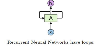
A: Neural Network

Xt: Input

ht: Output

The recurrence ensures a consistent flow of information. A (neural network block) generates output ht based on the input Xt.

An RNN can also be viewed as multiple copies of the same network, each passing information to its subsequent network.

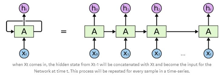
At each time step (t), the recurrent neuron receives input Xt from the previous time step ht-1 along with its own output.

If you want to dive deeper into RNNs, I highly recommend some good resources, including:

• Introduction to Recurrent Neural Networks.【2】

• Recurrent Neural Networks for Beginners.【3】

• Introduction to RNNs 【4】

RNNs have a significant drawback known as the vanishing gradient; that is, they struggle to learn long-distance dependencies (relationships between entities several steps apart).

Assuming the Bitcoin price in December 2014 was $350, we want to accurately predict the Bitcoin price in April and May 2018. Using RNNs, our model cannot accurately predict the prices over these months due to a lack of long-term memory. To address this issue, we developed a special type of RNN known as Long Short-Term Memory (LSTM).

What is Long Short-Term Memory?

This is a special neuron used to remember long-term dependencies. LSTM contains an internal state variable that is passed from one unit to another and modified by operation gates (Operation Gates) (which we will discuss in our example).

LSTMs are very clever; they can decide when to keep old information, when to remember and forget, and how to establish connections between old memories and new inputs. To gain a deeper understanding of LSTMs, here is a great resource: Understanding LSTM networks【5】.

Implementing LSTM

In our example, we will use LSTMs for time series analysis, predicting Bitcoin prices from December 2014 to May 2018. I have been using CryptoDataDownload【6】 because it is simple and intuitive. I used Google’s CoLab development environment because it is easy to set up and provides free GPU acceleration, reducing training time. If you are new to CoLab, here is a beginner’s guide【7】. The Bitcoin.csv file and all the code for this example can be obtained from my GitHub profile【8】.

What is Time Series Analysis?

Here, historical data is used to identify existing data patterns and utilize them to predict what will happen in the future. For a detailed understanding, refer to this guide【9】.

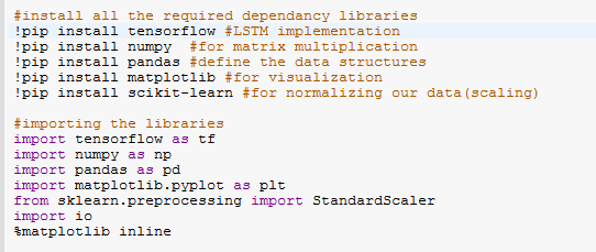
Import Libraries

We will work with various libraries that must first be installed in the CoLab notebook and then imported into our environment.

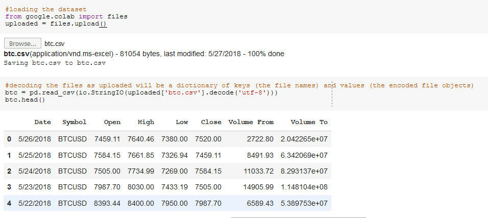
Loading Data

The btc.csv dataset contains Bitcoin prices and volumes, and we use the following command to load it into our working environment:

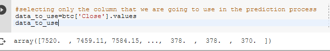
Target Variable

We will select the Bitcoin closing price as our target variable to predict.

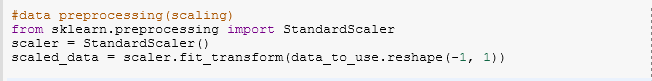
Data Preprocessing

Sklearn includes a preprocessing module that allows us to scale the data before feeding it into our model.

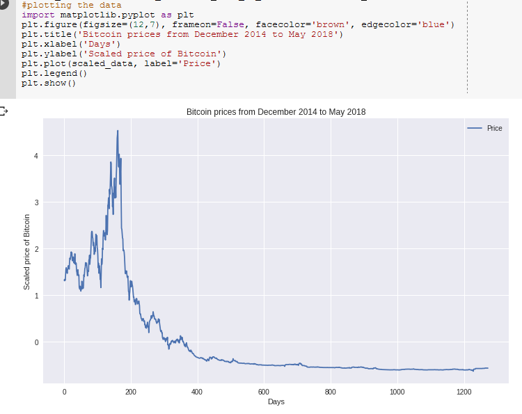
Plotting Data

Now let’s take a look at the trend of Bitcoin closing prices over a specific period.

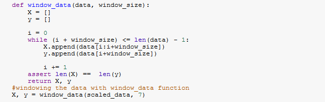
Feature and Label Dataset

This function is used to create features and labels for the dataset.

Input: data — The dataset we are using

Window_size — How many data points we will use to predict the next data point in the sequence (for example, if Window_size=7, we will use the previous 7 days to predict today’s Bitcoin price).

Outputs: X — The features split into windows of data points (if windows_size=1, x=[len(Data)-1, 1]).

y — labels — This is the next number in the sequence we are trying to predict.

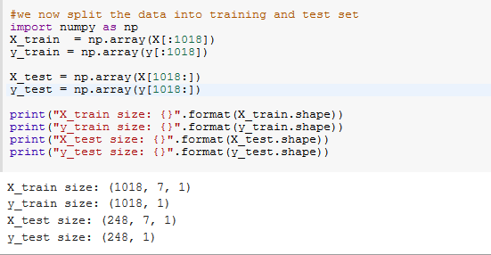
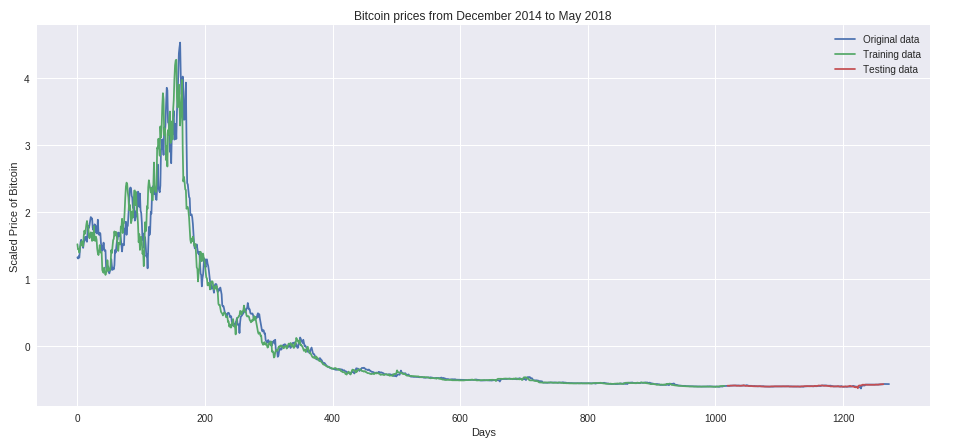
Training and Testing Datasets

Dividing the data into training and testing sets is crucial for getting a true estimate of model performance. We used 80% (1018) of the dataset as the training set, and the remaining 20% (248) as the validation set.

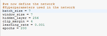
Defining the Network

Hyperparameters

Hyperparameters explain the high-level structural information of the model.

batch_Size — The number of data windows we pass at a time.

window_Size — The number of days we consider for predicting Bitcoin prices in our case.

hidden_layer — The number of units we use in the LSTM unit.

clip_margin — This is to prevent gradient explosion; we use a clipper to trim gradients above this margin. learning_rate — This is an optimization method aimed at reducing the loss function.

epochs — The number of iterations (forward and backward propagation) our model needs to perform.

You can customize various hyperparameters for your model, but for our example, let’s continue with the parameters we defined.

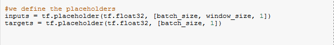
Placeholders

Placeholders allow us to send different data into the network using the tf.placeholder() command.

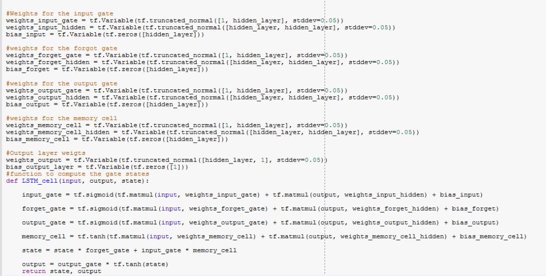
LSTM Weights

The weights of LSTM are determined by operation gates, including: Forget gate, Input gate, and Output gate.

Forget Gate

ft =σ(Wf[ht-1,Xt]+bf)

This is a sigmoid layer that combines the output from t-1 and the current input at time t into a single tensor, applies a linear transformation, and then performs a sigmoid operation.

Due to the presence of the sigmoid, the output of the gate is between 0 and 1. This number multiplies the internal state, which is why the gate is called the forget gate. If ft=0, the previous internal state is completely forgotten, while if ft=1, it is passed unchanged.

Input Gate

it=σ(Wi[ht-1,Xt]+bi)

This state combines the previous output with new input and passes them to another sigmoid layer. This gate returns a value between 0 and 1. The value of the input gate is then multiplied by the output of the candidate layer.

Ct=tanh(Wi[ht-1,Xt]+bi)

This layer applies the hyperbolic tangent to the mixture of the input and previous output, returning the candidate vector. The candidate vector is then added to the internal state, which is updated according to the following rule:

Ct=ft *Ct-1+it*Ct

The previous state is multiplied by the forget gate and then added to the score of the new candidate allowed by the output gate.

Output Gate

Ot=σ(Wo[ht-1,Xt]+bo)

ht=Ot*tanh Ct

This gate controls how much of the internal state is passed to the output and works similarly to the other gates.

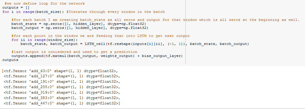
Network Cycle

A cycle is created for the network, iterating through each window in the batch, setting batch_states to all zeros. The output is used to predict Bitcoin prices.

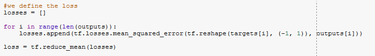
Defining the Loss Function

Here, we will use the mean_squared_error function to minimize the error.

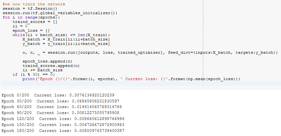
Training the Network

We now train the network with our initialized data and observe how the loss changes over time. The current loss decreases with the increase in observed time, improving the accuracy of our model for predicting Bitcoin prices.

Plotting Predictions

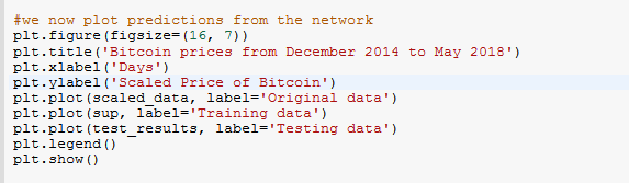
Output

Our model has been able to accurately predict Bitcoin prices based on the original data by implementing LSTM units. By reducing the window length from 7 days to 3 days, model performance can be improved. You can adjust the full code to optimize model performance.

Conclusion

I hope this article gives you a good start in understanding LSTMs.

1.https://www.kdnuggets.com/2016/11/quick-introduction-neural-networks

2.https://www.kdnuggets.com/2015/10/recurrent-neural-networks-tutorial

3.https://medium.com/@camrongodbout/recurrent-neural-networks-for-beginners-7aca4e933b82

4.http://www.wildml.com/2015/09/recurrent-neural-networks-tutorial-part-1-introduction-to-rnns

5.http://colah.github.io/posts/2015-08-Understanding-LSTMs

6.http://www.cryptodatadownload.com/

7.https://medium.com/deep-learning-turkey/google-colab-free-gpu-tutorial-e113627b9f5d

8.https://github.com/brynmwangy/predicting-bitcoin-prices-using-LSTM

9.https://www.kdnuggets.com/2018/03/time-series-dummies-3-step-process.html

Original link:

https://heartbeat.fritz.ai/a-beginners-guide-to-implementing-long-short-term-memory-networks-lstm-eb7a2ff09a27

-END-

Zhuanzhi · Know