Reprinted from Algorithm Advancement
With the popularity of models like Sora, diffusion, and GPT, deep generative models have once again become the focus of attention.
Deep generative models are a class of powerful machine learning tools that can learn the underlying distribution of input data and generate new sample data similar to the training data. They have been successfully applied in fields such as computer vision, density estimation, natural language processing, and speech recognition, providing a good paradigm for unsupervised learning.
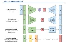
This article summarizes commonly used deep learning models and delves into their principles and applications: VAE (Variational Autoencoder), GAN (Generative Adversarial Network), AR (Autoregressive Model such as transformer), Flow (Flow Model), and Diffusion (Diffusion Model).
VAE (Variational Autoencoder)
Algorithm Principle:
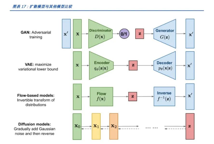
VAE is a deep generative model proposed based on autoencoders, combining variational inference and Bayesian theory. The goal of VAE is to learn a model that can generate samples similar to the training data. It assumes that the latent variables follow some prior distribution (such as standard normal distribution) and maps the input data to the posterior distribution of the latent variables through an encoder, then restores the latent variables back into generated samples through a decoder. The training of VAE involves optimizing two parts: reconstruction error and KL divergence.
Training Process:
-
Encoder: Encodes the input data x into the mean μ and standard deviation σ of the latent variable z.
-
Sampling: Samples an ε from the standard normal distribution, calculates z = μ + ε * σ.
-
Decoder: Decodes z into generated sample x’.
-
Calculates reconstruction error (such as MSE) and KL divergence, and optimizes model parameters to minimize their sum.
Advantages:
-
Can generate diverse samples.
-
Latent variables have a clear probabilistic interpretation.
Disadvantages:
-
The training process may be unstable.
-
The quality of generated samples may not be as good as other models.
Applicable Scenarios:
-
Data generation and interpolation.
-
Feature extraction and dimensionality reduction.
Python Example Code (Implemented using PyTorch):
import torch
import torch.nn as nn
import torch.optim as optim
class VAE(nn.Module):
    def __init__(self, input_dim, hidden_dim):
        super(VAE, self).__init__()
        self.encoder = nn.Sequential(
            nn.Linear(input_dim, hidden_dim),
            nn.ReLU(),
            nn.Linear(hidden_dim, 2 * hidden_dim)  # Mean and standard deviation
        )
        self.decoder = nn.Sequential(
            nn.Linear(hidden_dim, hidden_dim),
            nn.ReLU(),
            nn.Linear(hidden_dim, input_dim),
            nn.Sigmoid()  # For binary data, use Sigmoid activation function
        )
    def reparameterize(self, mu, logvar):
        std = torch.exp(0.5 * logvar)
        eps = torch.randn_like(std)
        return mu + eps * std
    def forward(self, x):
        h = self.encoder(x)
        mu, logvar = h.chunk(2, dim=-1)
        z = self.reparameterize(mu, logvar)
        x_recon = self.decoder(z)
        return x_recon, mu, logvar
# Example training process
model = VAE(input_dim=784, hidden_dim=400)
optimizer = optim.Adam(model.parameters(), lr=1e-3)
# Assuming x is the input data, batch_size is the size of the batch
x = torch.randn(batch_size, 784)
recon_x, mu, logvar = model(x)
loss = nn.functional.binary_cross_entropy(recon_x, x, reduction='sum') \
       + 0.5 * torch.sum(torch.exp(logvar) + mu.pow(2) - 1 - logvar)
optimizer.zero_grad()
loss.backward()
optimizer.step()
GAN (Generative Adversarial Network)
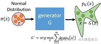
Algorithm Principle:
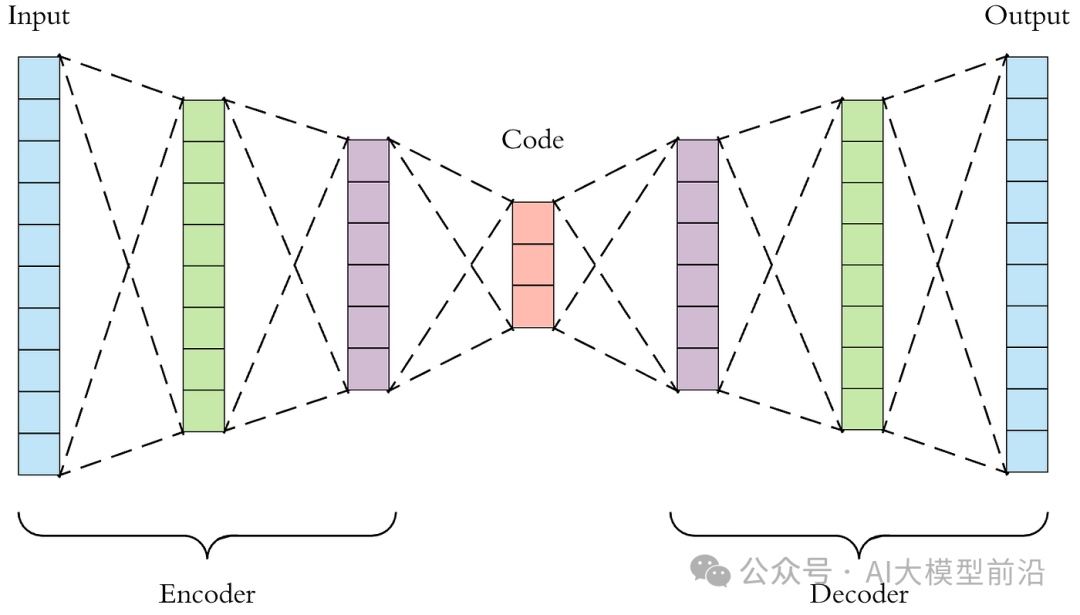
GAN consists of two parts: the generator and the discriminator. The generator’s task is to generate fake data that is as close as possible to real data, while the discriminator’s task is to distinguish whether the input data is real or generated by the generator. Both evolve together through competition and confrontation, ultimately allowing the generator to produce samples very close to real data.
Training Process:
-
The discriminator receives real data and fake data generated by the generator, performing binary classification training to optimize its ability to judge real or generated data.
-
The generator tries to generate more realistic fake data to deceive the discriminator based on the discriminator’s feedback.
-
Alternately train the discriminator and the generator until the discriminator cannot distinguish between real and generated data, or until a preset number of training epochs is reached.
Advantages:
-
Can generate high-quality samples.
-
The training process is relatively free and not limited by data distribution.
Disadvantages:
-
Training is unstable and can easily fall into local optima.
-
Requires a large amount of computational resources.
Applicable Scenarios:
-
Image generation.
-
Text generation.
-
Speech recognition, etc.
Python Example Code (Implemented using PyTorch):
import torch
import torch.nn as nn
import torch.optim as optim
# Discriminator
class Discriminator(nn.Module):
    def __init__(self, input_dim):
        super(Discriminator, self).__init__()
        self.fc = nn.Sequential(
            nn.Linear(input_dim, 128),
            nn.LeakyReLU(0.2),
            nn.Linear(128, 1),
            nn.Sigmoid()
        )
    def forward(self, x):
        return self.fc(x)
# Generator
class Generator(nn.Module):
    def __init__(self, input_dim, output_dim):
        super(Generator, self).__init__()
        self.fc = nn.Sequential(
            nn.Linear(input_dim, 128),
            nn.ReLU(),
            nn.Linear(128, output_dim),
            nn.Tanh()
        )
    def forward(self, x):
        return self.fc(x)
# Example training process
discriminator = Discriminator(input_dim=784)
generator = Generator(input_dim=100, output_dim=784)
optimizer_D = optim.Adam(discriminator.parameters(), lr=0.0002)
optimizer_G = optim.Adam(generator.parameters(), lr=0.0002)
criterion = nn.BCEWithLogitsLoss()
# Assuming real_data is the real data, batch_size is the size of the batch
real_data = torch.randn(batch_size, 784)
# Train the discriminator
for p in discriminator.parameters():
    p.requires_grad = True
for p in generator.parameters():
    p.requires_grad = False
noise = torch.randn(batch_size, 100)
fake_data = generator(noise)
real_loss = criterion(discriminator(real_data), torch.ones_like(real_data))
fake_loss = criterion(discriminator(fake_data.detach()), torch.zeros_like(real_data))
discriminator_loss = real_loss + fake_loss
optimizer_D.zero_grad()
discriminator_loss.backward()
optimizer_D.step()
# Train the generator
for p in discriminator.parameters():
    p.requires_grad = False
for p in generator.parameters():
    p.requires_grad = True
noise = torch.randn(batch_size, 100)
fake_data = generator(noise)
gen_loss = criterion(discriminator(fake_data), torch.ones_like(real_data))
optimizer_G.zero_grad()
gen_loss.backward()
optimizer_G.step()
AR (Autoregressive Model)
Algorithm Principle:
Autoregressive models are a type of generative model based on sequential data, which generate data by predicting the value of the next element in the sequence. Given a sequence (x_1, x_2, …, x_n), the autoregressive model tries to learn the conditional probability distribution (P(x_t | x_{t-1}, …, x_1)), where (t) represents the current position in the sequence. AR models can be implemented using structures like recurrent neural networks (RNN) or Transformers. Here, we analyze using Transformer as an example.
In the early stages of deep learning, convolutional neural networks (CNN) achieved significant success in image recognition and natural language processing. However, as the complexity of tasks increased, sequence-to-sequence (Seq2Seq) models and recurrent neural networks (RNN) became common methods for handling sequential data. Although RNNs and their variants perform well on some tasks, they often encounter gradient vanishing and model degradation issues when processing long sequences. To address these issues, the Transformer model was proposed. Subsequent large models like GPT and BERT are based on the Transformer and have achieved outstanding performance!
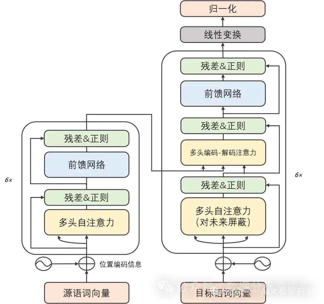
Model Principle:
The Transformer model cleverly combines the encoder and decoder into two main parts, each consisting of several identically constructed “layers” stacked together. These layers ingeniously combine self-attention sublayers with linear feedforward neural network sublayers. The self-attention sublayer cleverly employs a dot-product attention mechanism to weave unique representations for the input sequence at each position, while the linear feedforward neural network sublayer draws on the wisdom of the self-attention layer to produce informative output representations. Notably, both the encoder and decoder are equipped with a positional encoding layer specifically designed to capture the positional context within the input sequence.
Model Training:
The training of the Transformer model relies on backpropagation and optimization algorithms, such as stochastic gradient descent. During training, it meticulously calculates the gradient of the loss function with respect to the weights and employs optimization algorithms to fine-tune these weights in pursuit of minimizing the loss function. To accelerate training progress and improve the model’s generalizability, practitioners often adopt regularization techniques, ensemble learning, and other strategies.
Advantages:
-
Solves the issues of gradient vanishing and model degradation: The Transformer model, with its unique self-attention mechanism, can effortlessly capture long-term dependencies in sequences, thus freeing itself from the shackles of gradient vanishing and model degradation.
-
Exceptional parallel computing capability: The computational architecture of the Transformer model possesses inherent parallelism, allowing for rapid training and inference on GPUs.
-
Outstanding performance across multiple tasks: With strong feature learning and representation capabilities, the Transformer model exhibits exceptional performance in various tasks such as machine translation, text classification, and speech recognition.
Disadvantages:
-
High computational resource demands: Due to the parallel nature of the Transformer model’s computations, training and inference processes require substantial computational resources.
-
Sensitive to initialization weights: The Transformer model is quite picky about the choice of initialization weights; improper initialization can lead to unstable training or overfitting issues.
-
Limited handling of long-term dependencies: Although the Transformer model effectively addresses gradient vanishing and model degradation issues, it still faces challenges when dealing with extremely long sequences.
Application Scenarios:
The Transformer model has a wide range of applications in natural language processing, including machine translation, text classification, and text generation. Additionally, the Transformer model has also excelled in fields such as image recognition and speech recognition.
Python Example Code:
import torch
import torch.nn as nn
import torch.optim as optim
# This example is only for illustrating the basic structure and principles of the Transformer. Actual Transformer models (like GPT or BERT) are much more complex and require more preprocessing steps like tokenization, padding, masking, etc.
class Transformer(nn.Module):
    def __init__(self, d_model, nhead, num_encoder_layers, num_decoder_layers, dim_feedforward=2048):
        super(Transformer, self).__init__()
        self.model_type = 'Transformer'
        # encoder layers
        self.src_mask = None
        self.pos_encoder = PositionalEncoding(d_model, max_len=5000)
        encoder_layers = nn.TransformerEncoderLayer(d_model, nhead, dim_feedforward)
        self.transformer_encoder = nn.TransformerEncoder(encoder_layers, num_encoder_layers)
        # decoder layers
        decoder_layers = nn.TransformerDecoderLayer(d_model, nhead, dim_feedforward)
        self.transformer_decoder = nn.TransformerDecoder(decoder_layers, num_decoder_layers)
        # decoder
        self.decoder = nn.Linear(d_model, d_model)
        self.init_weights()
    def init_weights(self):
        initrange = 0.1
        self.decoder.weight.data.uniform_(-initrange, initrange)
    def forward(self, src, tgt, teacher_forcing_ratio=0.5):
        batch_size = tgt.size(0)
        tgt_len = tgt.size(1)
        tgt_vocab_size = self.decoder.out_features
        # forward pass through encoder
        src = self.pos_encoder(src)
        output = self.transformer_encoder(src)
        # prepare decoder input with teacher forcing
        target_input = tgt[:, :-1].contiguous()
        target_input = target_input.view(batch_size * tgt_len, -1)
        target_input = torch.autograd.Variable(target_input)
        # forward pass through decoder
        output2 = self.transformer_decoder(target_input, output)
        output2 = output2.view(batch_size, tgt_len, -1)
        # generate predictions
        prediction = self.decoder(output2)
        prediction = prediction.view(batch_size * tgt_len, tgt_vocab_size)
        return prediction[:, -1], prediction
class PositionalEncoding(nn.Module):
    def __init__(self, d_model, max_len=5000):
        super(PositionalEncoding, self).__init__()
        # Compute the positional encodings once in log space.
        pe = torch.zeros(max_len, d_model)
        position = torch.arange(0, max_len).unsqueeze(1).float()
        div_term = torch.exp(torch.arange(0, d_model, 2).float() *
                             -(torch.log(torch.tensor(10000.0)) / d_model))
        pe[:, 0::2] = torch.sin(position * div_term)
        pe[:, 1::2] = torch.cos(position * div_term)
        pe = pe.unsqueeze(0)
        self.register_buffer('pe', pe)
    def forward(self, x):
        x = x + self.pe[:, :x.size(1)]
        return x
# Hyperparameters
d_model = 512
nhead = 8
num_encoder_layers = 6
num_decoder_layers = 6
dim_feedforward = 2048
# Instantiate model
model = Transformer(d_model, nhead, num_encoder_layers, num_decoder_layers, dim_feedforward)
# Randomly generated data
src = torch.randn(10, 32, 512)
tgt = torch.randn(10, 32, 512)
# Forward pass
prediction, predictions = model(src, tgt)
print(prediction)
Flow (Flow Model)
Algorithm Principle:
Flow models are a type of deep generative model based on invertible transformations. They convert simple distributions (such as uniform or normal distributions) into complex data distributions through a series of reversible transformations.
Training Process:
During training, the flow model learns the parameters of the reversible transformations by minimizing the loss function between samples in the latent space and real data.
Advantages:
-
Can efficiently perform sample generation and density estimation.
-
Has invertibility, facilitating backpropagation and optimization.
Disadvantages:
-
Designing suitable reversible transformations can be challenging.
-
For high-dimensional data, flow models may struggle to capture complex dependencies.
Applicable Scenarios: Flow models are suitable for tasks such as image generation, audio generation, and density estimation.
Python Example Code:
import torch
import torch.nn as nn
class FlowModel(nn.Module):
    def __init__(self, input_dim, hidden_dim):
        super(FlowModel, self).__init__()
        self.transform1 = nn.Sequential(
            nn.Linear(input_dim, hidden_dim),
            nn.Tanh()
        )
        self.transform2 = nn.Sequential(
            nn.Linear(hidden_dim, input_dim),
            nn.Sigmoid()
        )
    def forward(self, x):
        z = self.transform1(x)
        x_hat = self.transform2(z)
        return x_hat, z
Diffusion Model
The Diffusion Model is a type of deep generative model inspired by the diffusion process in physics. Unlike traditional generative models (like VAE, GAN), the Diffusion Model generates data by simulating the gradual diffusion of data from random noise to target data. This model has shown excellent performance in image generation, text generation, and audio generation.
Algorithm Principle:
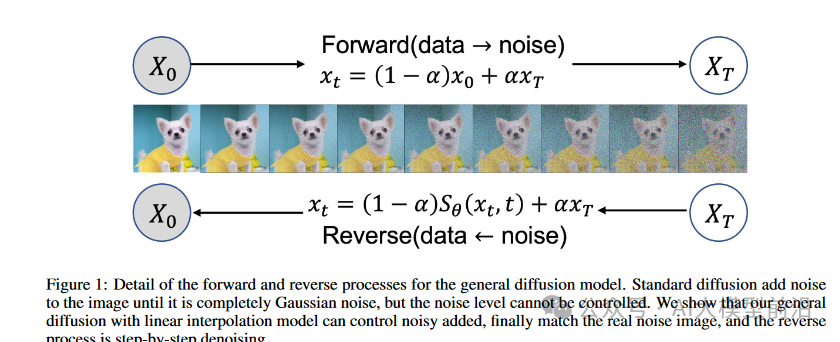
The basic idea of the Diffusion Model is to view the data generation process as a Markov chain. Starting from the target data, noise is gradually added at each step until reaching a pure noise state. Then, through a reverse process, data is gradually restored from pure noise back to the target data. This process is usually described by a series of conditional probability distributions.
Training Process:
-
Forward Process: Starting from real data, noise is gradually added until reaching a pure noise state. During this process, the noise level at each step needs to be calculated and saved.
-
Reverse Process: Starting from pure noise, noise is gradually removed until restored to target data. In this process, a neural network (usually a U-Net structure) is used to predict the noise level at each step and generate data accordingly.
-
Optimization: The model is trained by minimizing the difference between real data and generated data. Common loss functions include MSE (Mean Squared Error) and BCE (Binary Cross Entropy).
Advantages:
-
High generation quality: Because the Diffusion Model employs a gradual diffusion and restoration process, it can generate high-quality data.
-
Strong interpretability: The generation process of the Diffusion Model has clear physical meaning, making it easy to understand and explain.
-
Good flexibility: The Diffusion Model can handle various types of data, including images, text, and audio.
Disadvantages:
-
Long training time: Due to the multiple steps involved in diffusion and restoration, the training time is relatively long.
-
High computational resource demands: To ensure generation quality, the Diffusion Model typically requires substantial computational resources, including memory and computing power.
Applicable Scenarios:
The Diffusion Model is suitable for scenarios requiring high-quality data generation, such as image generation, text generation, and audio generation. Additionally, due to its strong interpretability and good flexibility, the Diffusion Model can also be applied in other areas requiring deep generative models.
Python Example Code:
import torch
import torch.nn as nn
import torch.optim as optim
# Define U-Net model
class UNet(nn.Module):
    # ... Model definition omitted ...
# Define Diffusion Model
class DiffusionModel(nn.Module):
    def __init__(self, unet):
        super(DiffusionModel, self).__init__()
        self.unet = unet
    def forward(self, x_t, t):
        # x_t is the data at the current time, t is the noise level
        # Use U-Net to predict noise level
        noise_pred = self.unet(x_t, t)
        # Generate data based on noise level
        x_t_minus_1 = x_t - noise_pred * torch.sqrt(1 - torch.exp(-2 * t))
        return x_t_minus_1
# Initialize model and optimizer
unet = UNet()
model = DiffusionModel(unet)
optimizer = optim.Adam(model.parameters(), lr=0.001)
# Training process
for epoch in range(num_epochs):
    for x_real in dataloader:  # Get real data from data loader
        # Forward process
        x_t = x_real  # Start from real data
        for t in torch.linspace(0, 1, num_steps):
            # Add noise
            noise = torch.randn_like(x_t) * torch.sqrt(1 - torch.exp(-2 * t))
            x_t = x_t + noise * torch.sqrt(torch.exp(-2 * t))
            # Calculate predicted noise
            noise_pred = model(x_t, t)
            # Calculate loss
            loss = nn.MSELoss()(noise_pred, noise)
            # Backpropagation and optimization
            optimizer.zero_grad()
            loss.backward()
            optimizer.step()
By analyzing and comparing the GAN, VAE, Flow, Diffusion, and AR five common generative models, we can see the advantages and disadvantages of different models and their applicable scenarios. VAE and GAN are two commonly used deep generative models, based on Bayesian probability theory and adversarial training to generate samples, respectively. The AR model is suitable for processing data with temporal dependencies, such as sequential data. Flow and Diffusion models exhibit good stability and diversity in sample generation, but require high computational costs. Future research on generative models may further explore model stability and trainability, as well as how to improve the quality and diversity of generated samples.