EdgeBERT: Limit Compression, 13 Times Lighter Than ALBERT!

Machine Heart Reprint

Source: Xixiaoyao’s Cute Selling House

Author: Sheryc_Wang Su

There are two types of highly challenging engineering projects in this world: the first is to maximize something very ordinary, like expanding a language model to write poetry, prose, and code like GPT-3; while the other is exactly the opposite, to minimize something very ordinary. For NLPers, this kind of “small project” is most urgently needed for BERT.

EdgeBERT: Limit Compression, 13 Times Lighter Than ALBERT!
From the 109M parameters of BERT in 2018, to the distilled DistilBERT with 52M parameters, then to TinyBERT with 14.5M parameters, and finally to ALBERT with 12M parameters that shares layers, the once cumbersome BERT that struggled to load parameters on clusters can now even run on mobile platforms. While we cheer for the lightweight BERT, a group of people have stepped forward—just running it on mobile is not enough! Their ideal is to run BERT on IoT devices, on low-power chips, on every electronic device we can touch!
This group of software and hardware geeks from Harvard/Tufts/HuggingFace/Cornell has now donned their robes, transforming into alchemists for extreme weight loss of BERT, adding many unexpected ingredients toward this seemingly impossible goal…
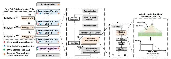
  • Paper Title: EdgeBERT: Optimizing On-Chip Inference for Multi-Task NLP

  • Paper Link: https://arxiv.org/pdf/2011.14203.pdf

Base Recipe: ALBERT
  • Source: ALBERT: A Lite BERT for Self-supervised Learning of Language Representations (ICLR’20)

  • Link: https://arxiv.org/pdf/1909.11942.pdf

EdgeBERT is optimized based on ALBERT.
ALBERT proposed by Google at ICLR’20 is currently the best compression scheme for BERT. Unlike previous methods that used knowledge distillation to obtain compressed models from the original BERT model (e.g., DistilBERT [1], TinyBERT [2]) or used floating-point quantization to obtain compressed models (e.g., Q8BERT [3]), ALBERT chooses to directly discard the pre-trained parameters of BERT, inheriting only the design philosophy of BERT. As the saying goes, “no breaking, no standing,” the ALBERT that inherits the soul of BERT achieves comparable performance to other BERT variants with only 12M parameters.
ALBERT made the following three improvements to BERT’s design:
  • Embedding Layer Decomposition: In BERT, the embedding dimension of WordPiece is consistent with the hidden layer dimension in the network. The authors propose that the embedding layer encodes context-independent information, while the hidden layer adds context information on this basis, so it should have a higher dimension; at the same time, if the embedding layer and hidden layer dimensions are consistent, increasing the hidden layer dimension will significantly increase the embedding layer parameter count. Therefore, ALBERT decomposes the embedding layer into matrices, introducing an additional embedding layer E. Let the vocabulary size of WordPiece be V, the embedding layer dimension be E, and the hidden layer dimension be H, then the embedding layer parameter count can be reduced from O(V x H) to O(V x E + E x H).

  • Parameter Sharing: In BERT, each Transformer layer has different parameters. The authors propose sharing all parameters of the Transformer layers across layers, thus compressing the parameter count to only the level of a single Transformer layer.

  • Next Sentence Prediction Task → Sentence Order Prediction Task: In BERT, in addition to the MLM task of the language model, there is also a next sentence prediction task, which judges whether sentence 2 is the next sentence of sentence 1. However, this task has been confirmed to have mediocre performance by models such as RoBERTa and XLNET. The authors propose replacing it with a sentence order prediction task, which judges the order of sentences 2 and 1 to learn text consistency.

ALBERT’s design is quite successful, becoming a classic example of compressing BERT, and starting from ALBERT to achieve the most extreme compression of BERT is indeed a good idea. ALBERT is already so powerful; how much further can EdgeBERT go? The authors immediately tantalize the readers with a comparison chart of memory usage/computation/performance on QQP. (Note: The vertical axis of memory usage is on a logarithmic scale!)
EdgeBERT: Limit Compression, 13 Times Lighter Than ALBERT!
This article utilizes ALBERT not only as initialization parameters but also for fine-tuning downstream tasks using a pre-fine-tuned ALBERT as a teacher for knowledge distillation to further enhance model performance.
Basic Recipe: Algorithm Optimization
EdgeBERT: Limit Compression, 13 Times Lighter Than ALBERT!
1. Entropy-Based Early Exit Mechanism
  • Source: DeeBERT: Dynamic Early Exiting for Accelerating BERT Inference (ACL’20)

  • Link: https://arxiv.org/pdf/2004.12993.pdf

ALBERT is good, but the Transformer is too deep, making it slow to compute; how about making it a bit shallower?
ACL’20’s DeeBERT proposes a dynamic early exit mechanism. This mechanism is designed to allow simple texts to undergo fewer computations while complex texts undergo more.
EdgeBERT: Limit Compression, 13 Times Lighter Than ALBERT!
In implementation, DeeBERT adds (n-1) “exit layer” classifiers (Early Exit Off-Ramps) to an n-layer BERT model. The exit layer classifier f_i is placed between the i-th and (i+1)-th layers of the Transformer as a marker to determine whether the information from the i-th layer of the Transformer is sufficient for inference. During inference, the entropy of the exit layer classifiers is calculated layer by layer starting from the bottom layer. When the entropy of an exit layer classifier at a certain layer is below a certain threshold, the result of that exit layer classifier is taken as the model result, saving subsequent layer computations.
EdgeBERT: Limit Compression, 13 Times Lighter Than ALBERT!
The above figure shows the average number of exit layers, theoretical time savings, and corresponding accuracy across four datasets (MNLI, QQP, SST-2, QNLI) with different entropy thresholds. After adding the early exit mechanism, when the accuracy loss is 1 percentage point, the theoretical running time can be reduced by 30%, 45%, 54%, and 36% on these four datasets, respectively; when the accuracy loss is 5 percentage points, the theoretical running time reduction can be further lowered to 44%, 62%, 78%, and 53% on these four datasets.
2. Dynamic Attention Span
  • Source: Adaptive Attention Span in Transformers (ACL’19)

  • Link: https://arxiv.org/pdf/1905.07799.pdf

ALBERT is good, but the attention range is too wide, making it slow to compute; how about narrowing it down a bit?
ACL’19’s Adaptive Attention proposes a dynamic attention span that attempts to reduce attention computation in this way. In the multi-head self-attention mechanism of the Transformer, different heads correspond to different attention ranges, and having each head perform attention calculations on all tokens undoubtedly adds unnecessary overhead. Therefore, Adaptive Attention adds a different mask for each head, allowing each token to only compute attention with surrounding tokens, thereby reducing the matrix computation overhead.
EdgeBERT: Limit Compression, 13 Times Lighter Than ALBERT!
Specifically, the mask function EdgeBERT: Limit Compression, 13 Times Lighter Than ALBERT! 
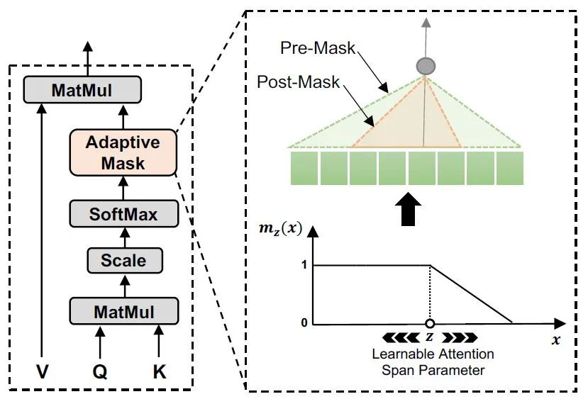
calculates attention weights based on the distance between two tokens using soft masking. The weights in the attention mechanism EdgeBERT: Limit Compression, 13 Times Lighter Than ALBERT! become:
EdgeBERT: Limit Compression, 13 Times Lighter Than ALBERT!
Where EdgeBERT: Limit Compression, 13 Times Lighter Than ALBERT! is a hyperparameter that controls the degree of soft masking, and EdgeBERT: Limit Compression, 13 Times Lighter Than ALBERT! is the length of the sequence up to token EdgeBERT: Limit Compression, 13 Times Lighter Than ALBERT! (the original text used a Transformer Decoder structure to learn the language model, so each token can only compute attention with its preceding tokens. In EdgeBERT, the formula is not mentioned, but based on the model diagram structure, the denominator should be modified to sum over the entire sequence). The boundary of the mask function EdgeBERT: Limit Compression, 13 Times Lighter Than ALBERT! will vary with the head-related parameters and the current input sequence: for each head in the attention mechanism EdgeBERT: Limit Compression, 13 Times Lighter Than ALBERT!, there are EdgeBERT: Limit Compression, 13 Times Lighter Than ALBERT! where EdgeBERT: Limit Compression, 13 Times Lighter Than ALBERT! and EdgeBERT: Limit Compression, 13 Times Lighter Than ALBERT! are trainable, and EdgeBERT: Limit Compression, 13 Times Lighter Than ALBERT! is a sigmoid function.
EdgeBERT even further simplifies Adaptive Attention: EdgeBERT: Limit Compression, 13 Times Lighter Than ALBERT! doesn’t even need to be calculated; directly assign each head a learnable EdgeBERT: Limit Compression, 13 Times Lighter Than ALBERT! without considering the input sequence, resulting in only 12 additional parameters EdgeBERT: Limit Compression, 13 Times Lighter Than ALBERT! 
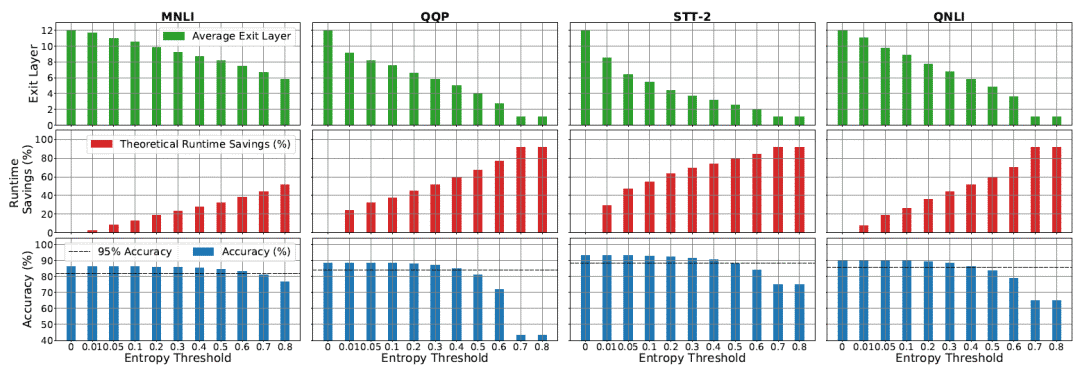
(because there are 12 heads). So what are the results of this approach? The authors pad/truncate all sequences to a length of 128, and through experiments, they obtained an astonishing result:
EdgeBERT: Limit Compression, 13 Times Lighter Than ALBERT!
The table shows the EdgeBERT: Limit Compression, 13 Times Lighter Than ALBERT! 
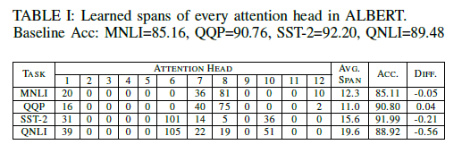
values of each head after optimization, and the model’s accuracy on the four tasks (MNLI/QQP/SST-2/QNLI). With most heads effectively masked (EdgeBERT: Limit Compression, 13 Times Lighter Than ALBERT!), the model surprisingly only lost 0.5 or even 0.05 in accuracy on these tasks! This method also brought the highest EdgeBERT: Limit Compression, 13 Times Lighter Than ALBERT! reduction in computation.
3. First-Order Network Pruning
  • Source: Movement Pruning: Adaptive Sparsity by Fine-Tuning (NeurIPS’20)

  • Link: https://arxiv.org/pdf/2005.07683.pdf

ALBERT is good, but storing parameters takes too much memory, making it costly; how about making it shorter?
This network pruning method uses a pruning algorithm for the model fine-tuning process from a NeurIPS’20 paper. The authors propose that the traditional zero-order network pruning (i.e., setting a threshold for the absolute values of parameters in the model, keeping those above it and zeroing those below) is not suitable for transfer learning scenarios, as the model parameters are mainly influenced by the original model but need to be fine-tuned and tested on the target task, so pruning based directly on the model parameters may lose knowledge from the source or target tasks. In contrast, the authors propose a Movement Pruning based on the first-order derivatives during the fine-tuning process: to retain parameters that deviate more from zero during fine-tuning.
Specifically: for model parameters EdgeBERT: Limit Compression, 13 Times Lighter Than ALBERT!, assign the same size importance scores EdgeBERT: Limit Compression, 13 Times Lighter Than ALBERT! to them, and the pruning mask EdgeBERT: Limit Compression, 13 Times Lighter Than ALBERT!.
During forward propagation, the neural network uses the parameters with the mask to compute the output components: EdgeBERT: Limit Compression, 13 Times Lighter Than ALBERT!
EdgeBERT: Limit Compression, 13 Times Lighter Than ALBERT!
During backpropagation, using the idea of the Straight-Through Estimator[4], approximate the loss function EdgeBERT: Limit Compression, 13 Times Lighter Than ALBERT! to obtain the gradient of the importance scores EdgeBERT: Limit Compression, 13 Times Lighter Than ALBERT!:
EdgeBERT: Limit Compression, 13 Times Lighter Than ALBERT!
For model parameters, we have:
EdgeBERT: Limit Compression, 13 Times Lighter Than ALBERT!
After substituting the above two expressions, the omitted mask matrix can be obtained:
EdgeBERT: Limit Compression, 13 Times Lighter Than ALBERT!
According to gradient descent, when EdgeBERT: Limit Compression, 13 Times Lighter Than ALBERT! is positive, the importance EdgeBERT: Limit Compression, 13 Times Lighter Than ALBERT! increases, indicating that only when positive parameters increase or negative parameters decrease during backpropagation will a larger importance score be obtained, avoiding pruning.
4. Zero-Order Network Pruning
  • Source: Deep Compression: Compressing Deep Neural Networks with Pruning, Trained Quantization and Huffman Coding (ICLR’16)

  • Link: https://arxiv.org/pdf/1510.00149.pdf

It may be shorter, but it feels like it hasn’t been pruned well enough; how about using another algorithm to make it even shorter?
This method is very simple: set an absolute value threshold for the parameters in the model, keeping those above it and zeroing those below. Since the method is so simple, it can be easily understood without formulas EdgeBERT: Limit Compression, 13 Times Lighter Than ALBERT!
EdgeBERT: Limit Compression, 13 Times Lighter Than ALBERT!
The comparison of the effects of first-order and zero-order network pruning is shown in the above figure (MvP: First-Order Network Pruning, MaP: Zero-Order Network Pruning). When the parameter sparsity is higher, first-order pruning performs better, while in other cases, simple zero-order pruning is more effective. At the same time, the research also found that when 95% of the embedding layer parameters are pruned, the model surprisingly maintains at least 95% accuracy on all four tasks.
5. Dynamic Floating-Point Quantization
  • Source: AdaptivFloat: A Floating-point based Data Type for Resilient Deep Learning Inference (arXiv Preprint)

  • Link: https://arxiv.org/pdf/1909.13271.pdf
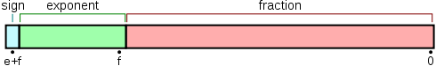
Hey, is there more? The network’s computation and storage processes have been optimized in terms of depth, width, and length; can the model still be lighter?
Indeed, up to this point, a typical alchemist would feel a sense of accomplishment looking at their three-dimensional pruned model, but this is still far from the goal of running BERT on all devices. The next part will delve into the fourth dimension—hardware optimization, which general NLP engineers rarely see. Before diving into hardware optimization, let’s start with a software appetizer and see how to optimize storage through floating-point quantization!
When we consider using the characteristics of floating-point numbers for computational acceleration, we first think of using FP16 mixed precision. While effective, it inevitably loses information, and the performance is somewhat affected. If we want to retain precision while accelerating training and reducing storage, we have to delve deeper and modify the representation of floating-point numbers!
This is precisely the intention of AdaptivFloat: to design a floating-point data type more suitable for deep learning scenarios. However, explaining the AdaptivFloat data type requires some knowledge unrelated to machine learning.
EdgeBERT: Limit Compression, 13 Times Lighter Than ALBERT!
According to the IEEE 754 binary floating-point standard, the binary representation of a floating-point number consists of three fields: sign bit (Sign, S), exponent bias (Exponent bias, E), and fraction value (Fraction, or Mantissa, F). Thus, a number can be represented as EdgeBERT: Limit Compression, 13 Times Lighter Than ALBERT!.
At this point, you might notice something strange: using the method of representing unsigned integers to take the exponent bias can only yield positive numbers! What about negative powers of 2? This is precisely why it is called “exponent bias”: it does not represent the exponent of 2 itself, but rather requires an additional constant to be added to represent the exponent of 2: EdgeBERT: Limit Compression, 13 Times Lighter Than ALBERT!.
Our commonly used floating-point numbers ensure that EdgeBERT: Limit Compression, 13 Times Lighter Than ALBERT! selection allows EdgeBERT: Limit Compression, 13 Times Lighter Than ALBERT! to be distributed almost evenly on both sides of the number line (for example, in 32-bit floating-point FP32, the exponent range is to), but such numbers as parameters for machine learning models are clearly not suitable: to increase the precision of fractions, we even have to allow EdgeBERT: Limit Compression, 13 Times Lighter Than ALBERT! numbers that clearly will not occur, which is really a waste of memory!
The key motivation for AdaptivFloat lies here: dynamically modifying EdgeBERT: Limit Compression, 13 Times Lighter Than ALBERT! based on model parameters. The so-called dynamic means that each tensor can receive a custom EdgeBERT: Limit Compression, 13 Times Lighter Than ALBERT!. The method is also simple: find the largest number in the tensor and ensure that it can be covered by the exponent range. However, saying it’s simple requires many other modifications to the existing floating-point representation to achieve this method, so if you’re interested, you can check out the original AdaptivFloat paper, and also refer to the IEEE 754 standard [5]!
EdgeBERT: Limit Compression, 13 Times Lighter Than ALBERT!
The results in the above image show that the Bit Width is the total number of bits of the floating-point number, and the last five rows used AdaptivFloat in the model with the exponent bias limited to 3 bits. Not comparing would not know; who would have thought that modifying a quantization method could directly beat FP32 on four datasets using only 8 bits?! Not only saving 3/4 of memory but also achieving better performance, perhaps this is the romance of geeks challenging the limits?
Advanced Recipe: Storage Medium Selection
Just optimizing software is not enough! If software optimization were sufficient, why buy SSDs or change GPUs (not)?
The purpose of EdgeBERT is to minimize inference latency and energy consumption when using BERT in edge computing scenarios. To maximize latency reduction, it is necessary to select the most efficient storage medium for different components of the network based on their read/write needs.
A major feature of BERT-like models is that they are all pre-trained models: these models are not plug-and-play but need to be fine-tuned on the target task before use. This gives these models two types of storage requirements:
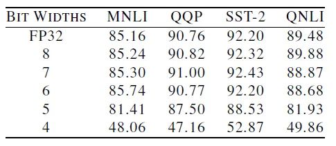
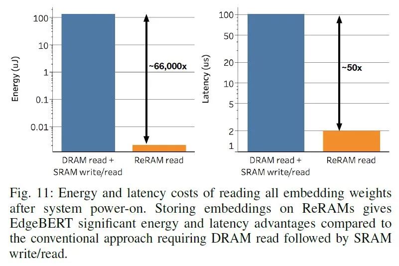
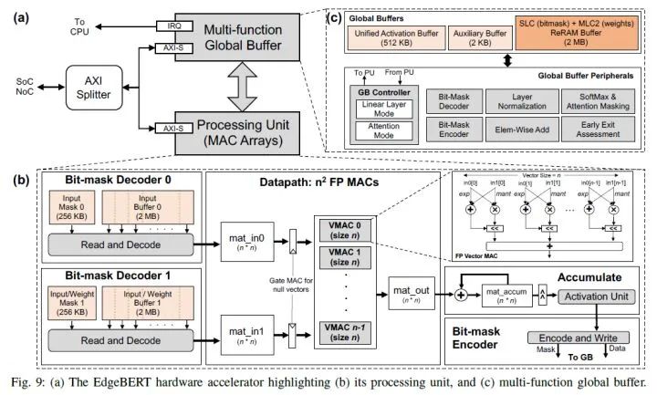
  • Embedding Layer: Stores the embedding vectors. EdgeBERT generally does not modify the embedding layer during downstream task fine-tuning. These parameters are equivalent to read-only parameters, requiring high-speed reading and hoping to retain original data during power loss to reduce data read/write overhead, so low-energy, fast-reading eNVM (Embedded Non-Volatile Memory) is suitable. The choice here is MLC-based ReRAM, a low-power, high-speed RAM.

  • Other Parameters: These parameters need to be changed during fine-tuning. SRAM is used here (unlike computer memory DRAM, SRAM is more expensive but consumes less power and has higher bandwidth, often used to make cache or registers).

EdgeBERT: Limit Compression, 13 Times Lighter Than ALBERT!
What impact does using ReRAM for the embedding layer bring? The results in the above image indicate that merely changing the hardware medium of the embedding layer can lead to approximately reduced inference latency and reduced energy consumption! This is a qualitative change in edge computing scenarios! (Why does ReRAM only read, while DRAM needs to calculate DRAM read + SRAM read/write? Because the ReRAM here is a specially designed read-only structure and can be directly read into the processor for computation. In contrast, DRAM, which is the general memory used in computers, needs to go through SRAM-based processor caches, so the read/write overhead needs to include this part of the read/write overhead.)
Combined Results
Alright, the results of using all the basic recipes individually have come out! So what results can be produced by combining them all?
EdgeBERT: Limit Compression, 13 Times Lighter Than ALBERT!
This figure shows the performance, computation, and memory usage of the complete EdgeBERT across four datasets. Among them, all red dot experimental configurations refer to the table above (i.e., TABLE IV).
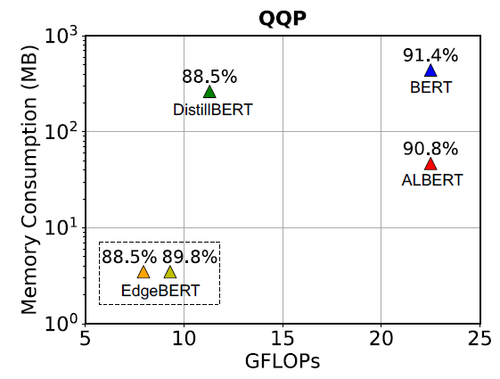
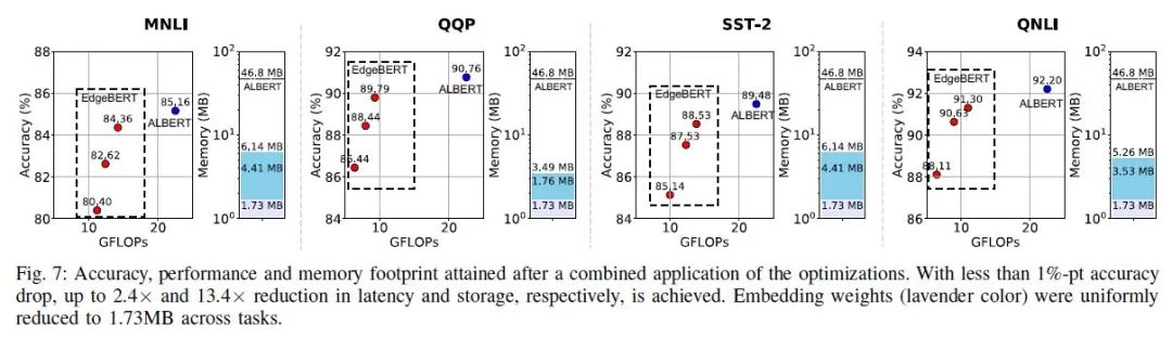
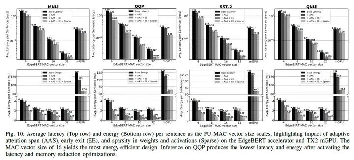
  • When the performance (accuracy) decreases by 1 percentage point compared to ALBERT, EdgeBERT can achieve reduced memory and inference speed; when the decrease is 5 percentage points, it can even achieve a reduction in inference speed.

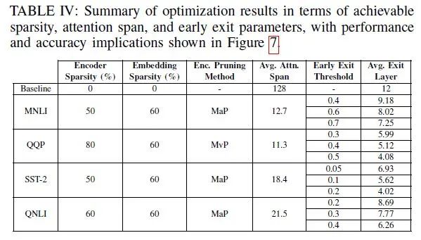
  • The embedding has been pruned to retain only 40%, resulting in the storage of the embedding layer parameters in eNVM being only 1.73MB.

  • The Transformer parameters of QQP have been masked by 80%, while those of MNLI, SST-2, and QNLI have been masked by 60% with only a 1 percentage point drop in performance.

Ultimate Recipe: Hardware Accelerator
What is this thing? Let me show you Google’s custom TPU accelerator for Raspberry Pi Coral:
EdgeBERT: Limit Compression, 13 Times Lighter Than ALBERT!
The hardware accelerator exclusive to EdgeBERT should be somewhat similar.
This part is completely not Wang Su’s expertise… Here’s a hardware structure diagram of the EdgeBERT accelerator:
EdgeBERT: Limit Compression, 13 Times Lighter Than ALBERT!
Those interested can refer to the original text for learning _(:з」∠)_
What is the use of this accelerator? It is a custom accelerator based on the operational characteristics of EdgeBERT, capable of fully accommodating the fine-tuned EdgeBERT for computation. As for the operational effects, they modified the length of the VMAC sequence (the unit sequence for matrix computation) in the model diagram and compared inference time and energy consumption with NVIDIA’s mobile TX2 mGPU:
EdgeBERT: Limit Compression, 13 Times Lighter Than ALBERT!
The hardware accelerator proposed in this article can bring energy savings compared to baseline hardware accelerators, and even achieve energy savings compared to NVIDIA’s TX2 mobile GPU! The energy-consuming BERT family finally has a day when it can be said to be “energy-saving”!
Conclusion
Compressing BERT is a research endeavor, but extreme compression of BERT is a challenging engineering task: whether it is the comprehensive pruning of the Transformer model, the trade-offs in read/write performance and fault tolerance of hardware storage media, or the design of dedicated hardware accelerators, any one of these is difficult enough, and combining them can lead to conflicts and even reverse optimization. This article tests the performance of several existing optimization methods in edge computing scenarios through extensive experiments, compares the differences between different optimization methods, analyzes the impacts and effects of all optimization methods when combined, and further proposes a dedicated hardware structure, achieving plug-and-play for the lightest BERT variant currently available. For scenarios requiring long standby, low power consumption, and low latency, such as smart homes or other IoT devices requiring NLP technology support, we may indeed see solutions similar to EdgeBERT accelerators in the not-too-distant future.
While we are still exploring model structures that may bring greater changes, from a practical perspective, using BERT optimization methods based on the Lottery Ticket Hypothesis[6] to find a better BERT-like substructure is still a good topic, as it allows more people, more often, and in more scenarios to use powerful pre-trained models. Do the optimization methods mentioned in this article inspire you to think?
Author Introduction
A top graduate from the CS program at Beihang University, a prospective Ph.D. at the University of Montreal/MILA, a senior ACG enthusiast, currently an intern at Tencent Tianyan Laboratory conducting NLP research. Although specializing in NLP, I am curious about all systems and directions that move towards more perfect intelligence. If one day N can truly understand my words, this world should be conquered by cuteness. (I haven’t published anything yet) Zhihu ID: Sheryc
References:
[1] Sanh et al. DistilBERT, a Distilled Version of Bert: Smaller, Faster, Cheaper and Lighter. In NeurIPS’19 EMC2 Workshop. https://arxiv.org/pdf/1910.01108.pdf
[2] Jiao et al. TinyBERT: Distilling BERT for Natural Language Understanding. In Findings of EMNLP’20. https://arxiv.org/pdf/1909.10351.pdf
[3] Zafrir et al. Q8BERT: Quantized 8Bit BERT. In NeurIPS’19 EMC2 Workshop. https://arxiv.org/pdf/1910.06188.pdf
[4] Bengio et al. Estimating or Propagating Gradients Through Stochastic Neurons for Conditional Computation. arXiv Preprint. https://arxiv.org/pdf/1308.3432.pdf
[5] IEEE 754 – Wikipedia. https://zh.wikipedia.org/wiki/IEEE_754
[6] Frankle et al. The Lottery Ticket Hypothesis: Finding Sparse, Trainable Neural Networks. In ICLR’19. https://arxiv.org/pdf/1803.03635.pdf
AAAI 2021 Online Sharing | Using Multi-Round Reading Comprehension Framework to Solve Entity Linking Problems
In a paper accepted by the AAAI 2021 conference at Huawei Cloud, researchers proposed using a multi-round reading comprehension framework to solve the entity linking problem for short texts, achieving the current SOTA entity linking effect on multiple Chinese and English datasets.
On January 14, 20:00,Huawei Cloud Voice Semantic Innovation Lab algorithm engineer Xavier will provide a detailed interpretation of this cutting-edge research.
Add the Machine Heart assistant (syncedai5), note “AAAI”, and join the group to watch the live broadcast together.
EdgeBERT: Limit Compression, 13 Times Lighter Than ALBERT!

© THE END

Reprint please contact this public account for authorization

Submission or seeking coverage: [email protected]

Leave a Comment