DNN/LSTM/Text-CNN Sentiment Classification Practice and Analysis

Follow the public account “ML_NLP”

Set as “Starred”, heavy content delivered at the first time!

Author: Tian Yu Su

Zhihu: https://zhuanlan.zhihu.com/p/37978321

Editor: Wang Meng, City University of Macau (Deep Learning Go Go Go public account)

This article is for academic sharing only. If there is any infringement, please contact the backend to delete the article.

Introduction

I recently reviewed Yoon Kim’s 2014 paper “Convolutional Neural Networks for Sentence Classification”. I have to say that although the Text-CNN approach is relatively simple, it can indeed achieve good results in Sentence Classification. Additionally, previously

@Howard

raised the question:

Why is LSTM so effective?www.zhihu.com

At that time, I shared some thoughts based on my understanding. The expert also clarified the experimental results of models such as DNN, CNN, and RNN in the question. So I have always wanted to try how these models perform in practice, and thus this article came about by chance.

This article will use a publicly available dataset from Cornell (which is also one of the datasets used in Yoon Kim’s paper experiments). The data link is as follows:

Datawww.cs.cornell.edu

The data is also available in my GitHub, so if you pull the code, you won’t need to download the data separately~

This dataset is used for sentiment classification and contains 5331 positive texts and 5331 negative texts. All the following code will be based on this data to construct a sentence classification model.

TensorFlow version for code execution: 1.6.0

Main Content

The article is divided into 6 parts:

• Data Processing
• DNN Model
• LSTM Model
• Text-CNN Model
• Text-CNN Model (Advanced Version)
• Model Results Comparison and Analysis

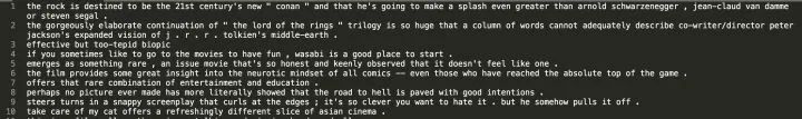
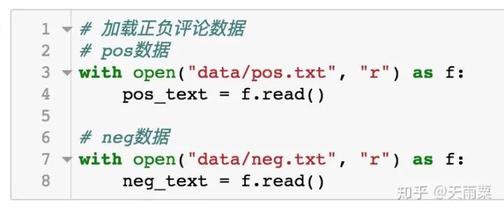
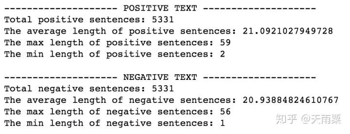
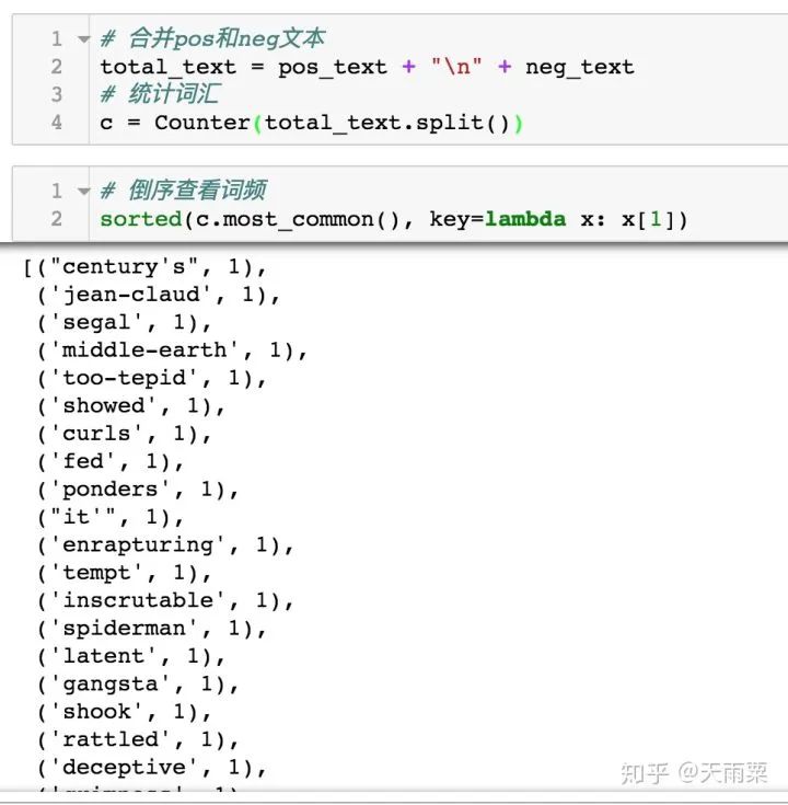
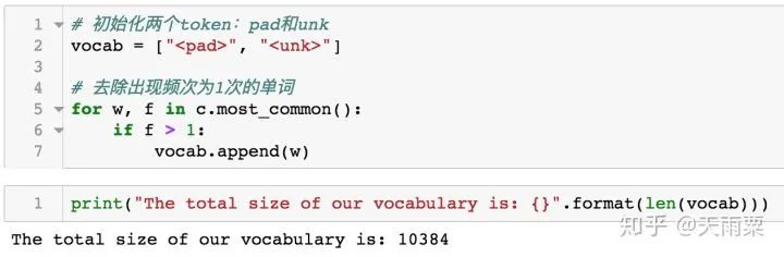
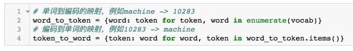
It is recommended to pull the code for supplementary learning~

1. Data Processing

The data we use has undergone some preprocessing, and we can open the txt document to check the content:

Each line is a complete sentence, with sentences separated by spaces.

Our data processing phase is to convert these texts into tokens that machines can recognize.

1. Load Data

First, we will load the data:

Descriptive statistics of the text:

We can see that our positive and negative comment texts each have 5331 entries, with an average length of about 20.

2. Construct Dictionary

Next, we need to construct our dictionary based on this corpus. The steps for constructing the dictionary generally involve tokenizing the text and then deduplicating. When we count the words in the text, we find that many words appear only once. These words will increase the capacity of our dictionary and also introduce some noise into the text processing.

It can be found that many words appear only once. Removing these words will greatly reduce our dictionary capacity and speed up model training, while also reducing some noise.

In practice, after tokenization, words are usually stemmed, and then word frequency statistics are performed. Here, I am doing it rather roughly~

Therefore, in the process of constructing the dictionary, we only keep words that appear more than once in the corpus. The and are two initialized tokens, where is used for sentence padding and is used to replace words that did not appear in the corpus. Finally, we obtain a dictionary containing 10384 words.

3. Construct Mapping

With the dictionary, we need to construct mappings from word to token and from token to word:

4. Convert Text

With the mapping tables, we can convert the original text into machine-readable encoding. In addition, to ensure that sentences have the same length, we need to process the sentence length. We can see in the descriptive statistics phase that the average length of sentences in the corpus is 20 words, so we set 20 as the standard length for sentences:

• Truncate sentences that exceed 20 words;
• PAD complete sentences that are less than 20 words.

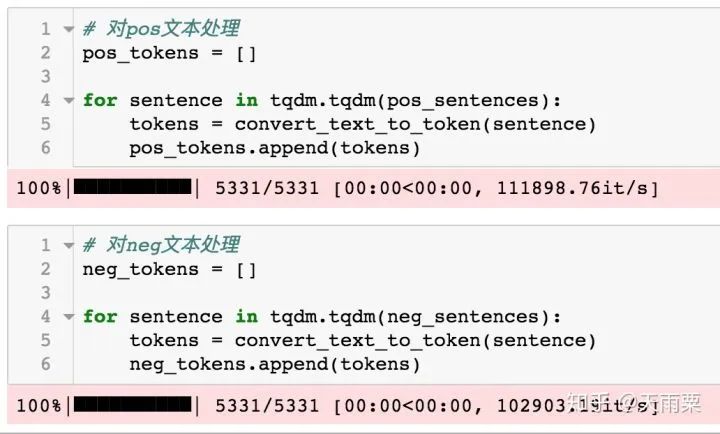
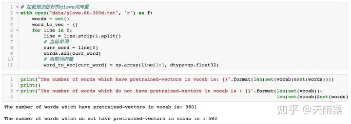
Next, we construct a function that can receive a complete str type sentence and convert it into tokens based on the mapping table.

In this function, we first need to get the encoding for and for later sentence conversion. Next, we map the sentence, replacing any unseen words with the token. Finally, we standardize the length of the sentence.

Next, we convert the pos and neg texts respectively:

5. Load Pre-trained Word Vectors

This article will use the pre-trained 300-dimensional word vectors from Glove as the model’s word embeddings.

Since this file is too large, I did not submit it to GitHub. Please download the dataset from the Glove official website: Global Vectors for Word Representation or click here to download the Glove.6B link directly. After downloading, unzip the compressed package and place glove.6B.300d.txt in the data directory.

We will load this word vector:

It can be seen that among the words in our constructed dictionary, 9801 words have pre-trained word vectors, while 583 words do not have corresponding pre-trained word vectors. Yoon Kim mentioned in the paper that for these words without word vectors, they can be replaced with random values.

Therefore, we will construct a matrix of size vocab_size * embedding_size based on the pre-trained word embeddings.

The above code execution will yield a static_embeddings matrix, where each row corresponds to the word vector (300 dimensions) of a word in the dictionary.

So far, we have basically completed the data preprocessing part. In this part, we mainly completed two main tasks:

• Converted the original text into tokens
• Constructed our word embeddings

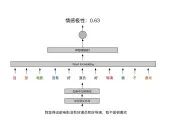
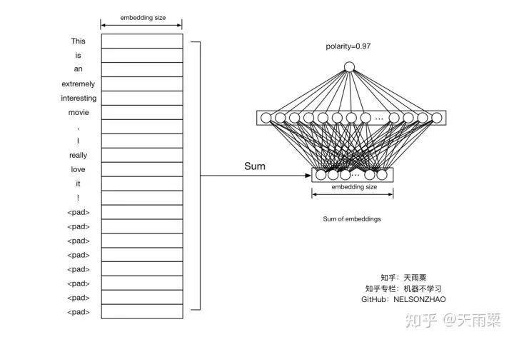
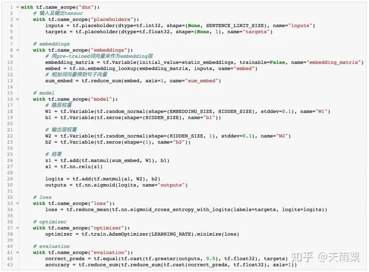
2. DNN Model

1. Model Structure

The DNN model processes sentences in a very simple way. For each word in the sentence, it first obtains the word vector, then sums these word vectors to obtain the sentence vector. This vector is then connected to a fully connected layer, and finally the result is output at the output node. As shown in the figure below:

Our input is a sentence, “This is an extremely interesting movie, I really love it!”, and we use to pad the sentence length to 20. For each word, we perform word embedding to obtain a 20 * embedding_size matrix, and by summing all rows of this matrix, we get the sentence embedding, which is a vector of length embedding_size.

Then, this sentence embedding is connected to a fully connected layer, and finally a single node outputs the probability value.

2. Model Code

Based on the above model structure, we can define the following code:

In this code, I divided it into several scopes, each containing a set of operations. The following models will also adopt a similar coding approach.

• In placeholders, we define two tensors: inputs and targets, where inputs are our input with the shape [batch_size, sentence_len], and here our sentence_len is 20. Targets are either 1 or 0, with the shape [batch_size, 1]
• In embeddings, we define our embedding matrix, filled with pre-trained values. Since these word vectors are pre-trained, we explicitly specify trainable=False. After lookup, we obtain the word vectors for each word in our input sequence and sum them to get sum_embed.
• In model, we define the weights for the fully connected layer and output layer and calculate the result, using relu as the activation function for the fully connected layer.
• In loss, we define the sigmoid cross-entropy loss function.
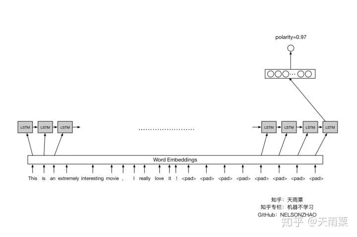
• In evaluation, we define an operation to calculate accuracy. Since our pos and neg samples are 1:1, if the predicted probability exceeds 0.5, we consider it positive; otherwise, it’s negative.

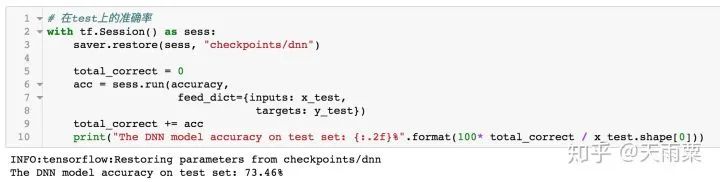
3. Train Model

After constructing the model, we set hyperparameters and train the model. In this model, I used 80% of the data for training and the remaining 20% for testing. The accuracy on train and test is plotted as follows:

Using the trained model to predict the test data, we obtain the accuracy as follows:

It can be seen that the DNN model has a certain degree of overfitting on train. As training progresses, when it reaches around 25 epochs, the model’s accuracy on train reaches 100%, and the accuracy on test stabilizes, with a final accuracy of 73.46% on test.

It is evident that the DNN model performs well, although this performance mainly comes from the word embeddings. The overfitting observed in the model can be alleviated by dropout or adding L2 regularization. You can try it yourself~

3. LSTM Model

1. Model Structure

The RNN model can handle sequential problems, and LSTM is particularly good at capturing long sequence relationships. Due to the presence of gates, LSTM can learn and grasp the forward and backward dependencies in sequences well, making it more suitable for handling long sequence NLP problems. The model structure is as follows:

After performing word embedding on the sentence, it is passed into the LSTM sequence for training. The last hidden state of LSTM is extracted and connected to a fully connected layer to obtain the final output result.

2. Model Code

Based on the LSTM structure mentioned above, we construct the model code as follows:

In the above code, there are several parts similar to those in DNN, which will not be repeated here.

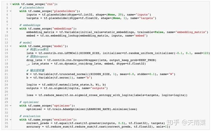
• In embeddings, unlike DNN where word vectors are summed, LSTM does not require summing word vectors but directly learns from the word vectors themselves. Whether summing or averaging, such aggregation operations will lose some information.
• In model, we first construct the LSTM unit and add dropout to prevent overfitting. After executing dynamic_rnn, we obtain the last state of LSTM, which is a tuple structure containing cell state and hidden state (the result after the output gate). We only take the hidden state output, i.e., lstm_state.h, and connect this vector to obtain the final output result.
• Optimizer and evaluation are similar to those in the DNN model and will not be repeated.

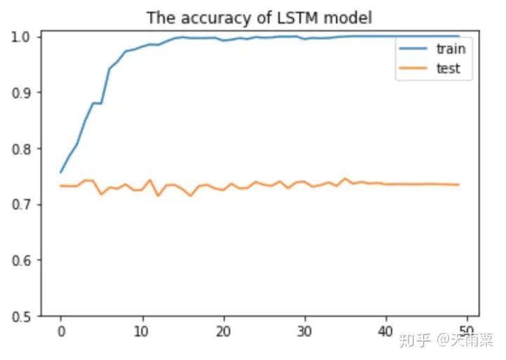
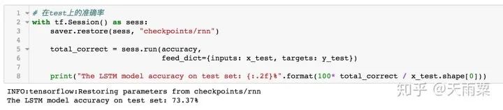
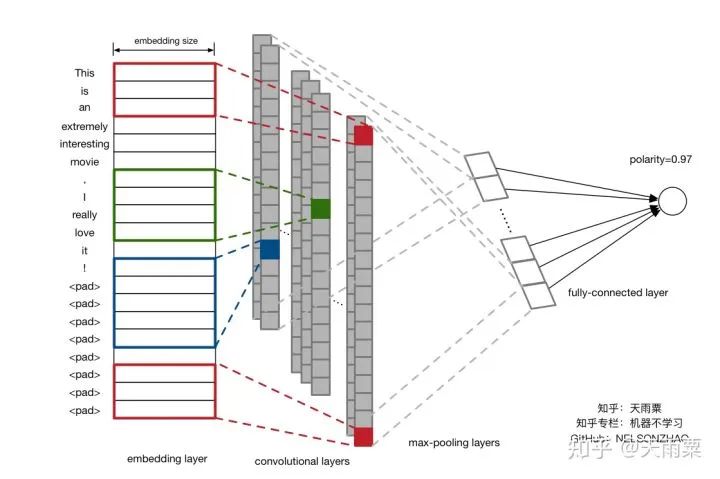
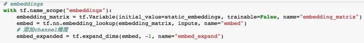
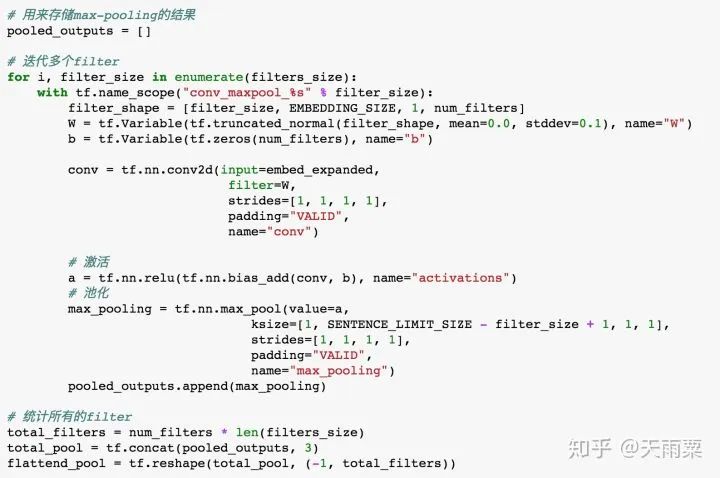
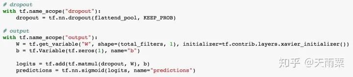
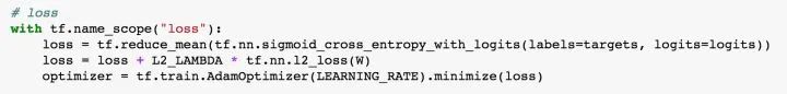
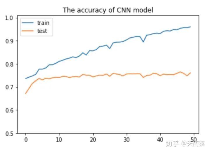
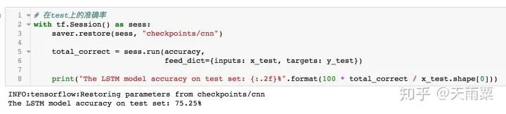
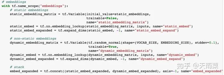
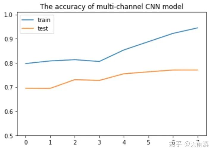
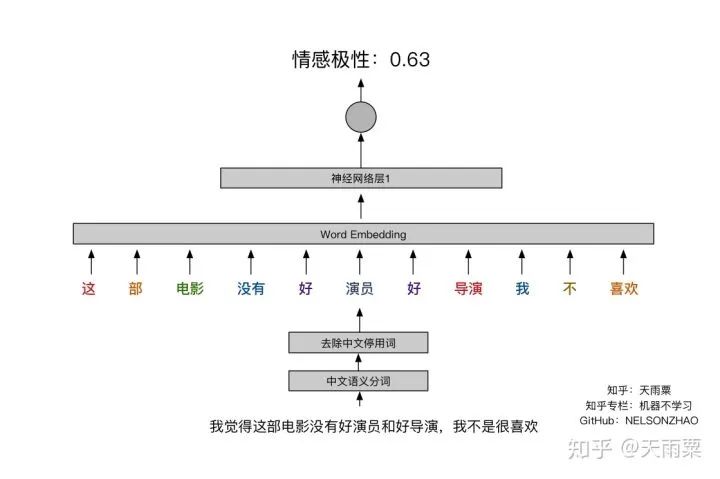
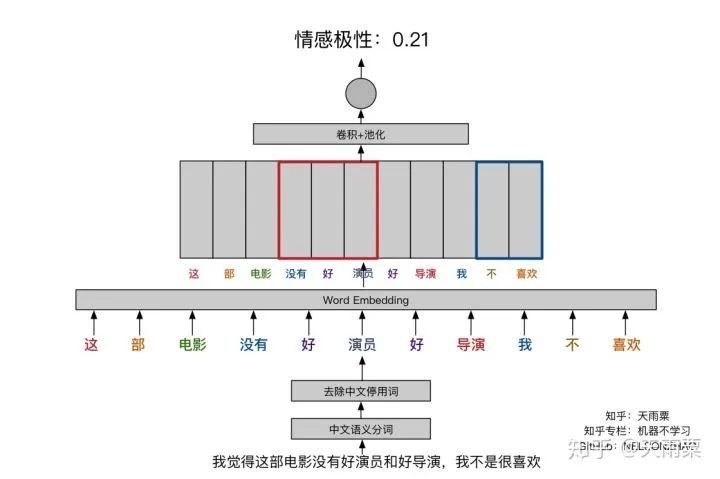
3. Train Model

After constructing the model, we set hyperparameters for training. Here, I used a single-layer LSTM with 512 nodes. The accuracy of training data and testing data for each epoch is plotted as follows:

Using the trained model to predict the test data, we obtain the accuracy as follows:

It seems that the results are not much different from DNN. LSTM appears to be overfitting, and I did not carefully tune the parameters~ Additionally, this also indicates that pre-trained word vectors have a significant effect on the DNN model, allowing it to approach LSTM’s accuracy. Furthermore, compared to DNN, the LSTM model converges faster on train.

4. CNN Model

1. Model Structure

Unlike LSTM, which captures long sequences, CNN captures local features. We all know that CNN has achieved good results in image processing because its convolution and pooling operations can capture local features in images. Similarly, CNN used in text processing can also capture local information in text. The implementation below refers to Yoon Kim’s 2014 paper on TextCNN. The model structure is as follows:

As shown in the figure above, assuming our sentence length is 20, we pad the insufficient ones with . After inputting the sentence sequence and performing embedding, we obtain the word vectors for each word (assuming the word vector dimension is 300), resulting in a sentence_len * embedding_size matrix, as shown in the embedding layer in the figure above. Here, we can treat it as a width=embedding_size, height=sentence_len, channel=1 image, and we can use filters to perform convolution operations.

Next, we adopt three types of filters. Yoon Kim mentioned in the paper that the three filter sizes are 3, 4, and 5, with 100 of each type. As shown in the figure above, the red filter has height=3, width=embedding_size, channel=1; the green has height=4, and the blue has height=5. So why do the filters keep the width consistent with the embedding_size? This is easy to understand; the width represents the size of the word vector. For a single word, splitting its word vector is meaningless. The purpose of the convolution operation is to slide in the height direction to capture the local relationships between words.

After the convolution operation, we obtain outputs from the convolutional layers as shown in the figure above, which are multiple column vectors. Then, we apply max-pooling to extract the most important information from each column vector. Finally, we connect a fully connected layer to obtain the output result.

2. Model Code

The code for TextCNN is actually quite simple. As long as we can construct that figure, we can directly complete the convolution operation according to the image.

Since the code is relatively long, we will look at each name_scope separately, and we will not repeat placeholders, evaluation, and other parts that are similar to DNN and LSTM; here we only explain the key parts of the code.

Complete code can be found on my GitHub

embeddings

First, the embeddings, which differ from DNN and LSTM by just one line of code. Because the convolution operation requires a channels dimension, after constructing the embed, the actual shape is (batch_size, vocab_size, embedding_size), but TensorFlow requires the dimensions for convolution to be (batch_size, heights, widths, channels). Therefore, we increase the channels dimension using expand_dims.

convolution-pooling

Since we used multiple filters (filter sizes=2, 3, 4, 5, 6), we need to handle convolution pooling operations separately for each filter. First, we define pooled_outputs to store the outputs of the convolution pooling operations for each filter.

For each filter, we first perform the convolution operation to get conv, then activate it with the relu function and perform pooling to get max_pooling. Since we have 100 of each filter, after flattening, we can obtain a 100*5=500-dimensional vector for connecting to the fully connected layer.

outputs

Yoon Kim mentioned in the paper that adding dropout can improve model performance, so we add dropout here. Finally, the output layer connects fully, passing through sigmoid activation to output the final result.

loss

Unlike previous models, here the loss adds L2 regularization on the fully connected layer weights W. Although Yoon Kim said that adding L2 is not critical, I found that adding L2 improves the model’s performance on test after trying it myself.

3. Train Model

After training the model, we can obtain the changes in accuracy on train and test, as shown in the figure below:

Since we added L2 regularization and dropout, we can see that the model does not overfit on train as much as DNN and LSTM, and after 50 epochs, the accuracy on train still has room for improvement. On test, the model stabilizes after about the 10th round.

Let’s use the model to predict the accuracy on test:

It can be seen that this accuracy is higher than that of DNN and LSTM models, with an accuracy of 75.25% on test. It is evident that this simple TextCNN model can achieve a relatively high accuracy.

5. Advanced CNN Model

1. Model Structure

The advanced CNN model adds an additional channel to the embedding compared to the TextCNN. In the fourth part, we constructed the shape=(sentence_len, embedding_size, 1) graph using pre-trained word embeddings. Since the pre-trained word embeddings are not trained within the model, we refer to them as static embeddings; Yoon Kim mentioned another type called non-static embedding, which requires the embedding layer to be trained along with the model. This layer can be randomly initialized or initialized with pre-trained word embeddings and fine-tuned to capture task-specific information. The specific model structure is as follows:

As can be seen, the difference between this model and the fourth part is that our embedding layer has two layers. That is, an additional non-static embedding is added on top of the static embedding, turning the original single-channel image into a two-channel image. The benefit of adding a non-static embedding is that the model can learn task-specific information through the corpus.

2. Model Code

Since this multi-channel model merely adds a trainable embedding to the model from the fourth part, I only provide the code for the embedding layer:

Here, in addition to the static embeddings, we also need to construct a non-static embedding, which we fill with random initialization. After obtaining these two embeddings, we can stack them along the channel dimension to obtain a tensor of shape=(sentence_len, embedding_size, 2).

The subsequent parts are the same as the one-layer channel model; note that the filter values in the channel direction should be set to 2.

3. Train Model

After training the model, we plot its accuracy changes on train and test as follows:

I only trained for 8 epochs because I found that further training would lead to severe overfitting. Since our training corpus is not large, adding another layer of embedding makes the model very prone to overfitting. Therefore, I set 8 epochs, which allows the model to achieve good results on test.

As shown in the figure above, the multi-channels model achieves an accuracy of 76.93% on test, higher than the previous three models.

6. Summary

Up to this point, we have completed the tasks of processing sentence classification using DNN, RNN, and CNN. Among them, the accuracy on test between DNN and RNN is quite similar, while CNN’s accuracy on test is 1% to 2% higher. The multi-channels CNN achieves an accuracy of 76.93% on test, with fewer training iterations.

Our models are relatively simple, but overall, all these models achieved good accuracy, largely due to the pre-trained word embedding. This highlights the importance of word embedding in NLP models, and the accuracy improvement of the multi-channels CNN comes from incorporating task-specific information.

Furthermore, let’s intuitively understand the differences between DNN, RNN, and CNN in NLP processing, taking sentiment analysis as an example.

First, DNN is the simplest model and does not handle sequential relationships, so it does not perform well in many NLP tasks, as shown in the figure below:

This sentence is inherently negative, but we know that DNN processes text by summing word vectors. Therefore, when the positive words in this sentence outnumber the negative ones, the model is easily misled. In the above sentence, there are 2 “good” and 1 “like”, while the negation words only include “not” and “no”, leading the model to mistakenly classify this as a positive sentence. However, in reality, “not” negates “good”, and “no” negates “like”.

Next, let’s discuss RNN (LSTM), as shown in the figure:

The advantage of RNN is that it can capture long sequence relationships, relying on gates to do so. Because of the presence of gates, the model learns which information to retain and which to forget. In processing, when the model sees “good”, it still remembers the preceding negation word “not”, and similarly learns the relationship between “like” and “not”.

Finally, let’s discuss CNN, as shown in the figure:

Although CNN does not have the sequential dependency structure of RNN, its convolution operation essentially captures local information, while pooling extracts the most important information from the local context. For example, the red box indicates a size=3 filter, and the blue box indicates a size=2 filter. They can capture local negation relationships such as “not-good actor” and “not-like”, thus also correctly classifying the sentence.

In summary, DNN cannot capture sequential relationships, RNN (LSTM) can capture long dependency relationships, and CNN can capture local sequential relationships.

Repository address shared:

Reply “code” to the backend of the Machine Learning Algorithm and Natural Language Processing public account to get 195 NAACL + 295 ACL 2019 papers with open-source code. The open-source address is as follows: https://github.com/yizhen20133868/NLP-Conferences-Code

Big news! The Yizhen Natural Language Processing - Pytorch exchange group has been officially established! There are a lot of resources in the group, and everyone is welcome to join and learn!
Note: Please modify the remarks when adding to [School/Company + Name + Direction] For example - HIT + Zhang San + Dialogue System. The account owner, please consciously avoid. Thank you!

Recommended reading:
Longformer: A Pre-trained Model Born for Long Documents Beyond RoBERTa
An Intuitive Understanding of KL Divergence
Top 100 Must-Read Papers in Machine Learning: High Citation, Comprehensive Classification, Wide Coverage | GitHub 21.4k Stars