
Source: Pythonic Biologists
This article is about 7000 words, and it is recommended to read for 10+minutes. Is deep learning the same as classical statistics?
Is deep learning the same as classical statistics? Many people may have this question, as there are many similar terms between the two. In this article, theoretical computer scientist and renowned Harvard professor Boaz Barak compares the differences between deep learning and classical statistics in detail, arguing that “if deep learning is understood purely from a statistical perspective, key factors for its success will be overlooked.”
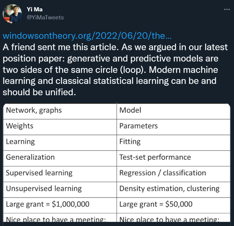
Image source: https://twitter.com/YiMaTweets/status/1553913464183091200
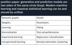
Deep learning (or general machine learning) is often considered a simple form of statistics, as it deals with concepts fundamentally similar to those studied by statisticians, but describes them using different terminologies. Rob Tibshirani summarized an interesting “glossary” as follows:
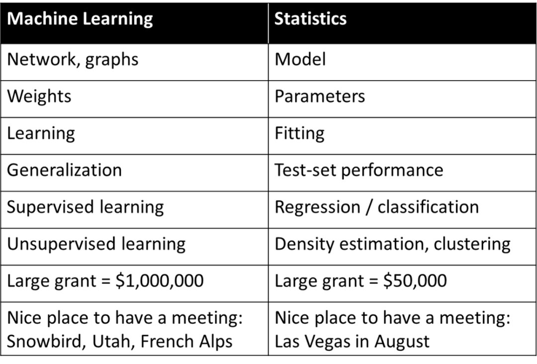
Does some of the content in the table resonate with you? In fact, everyone engaged in machine learning knows that many of the terms on the right side of Tibshirani’s published table are widely used in machine learning.
If deep learning is understood purely from a statistical perspective, key factors for its success will be overlooked. A more appropriate evaluation of deep learning is that it uses statistical terminology to describe completely different concepts.
A proper evaluation of deep learning is not that it uses different words to describe old statistical terms, but that it uses these terms to describe completely different processes.
This article will explain why the foundations of deep learning are actually different from those of statistics, and even different from classical machine learning. The article first discusses the differences between the “explanation” task and the “prediction” task when fitting a model to data. Then it discusses two scenarios of the learning process:
1. Fitting statistical models using empirical risk minimization;
2. Teaching students mathematical skills. The article then discusses which scenario is closer to the essence of deep learning.
Although the mathematics and code of deep learning are almost identical to fitting statistical models, on a deeper level, deep learning is more like the scenario of teaching students mathematical skills. Moreover, few would dare to claim: I have mastered the complete theory of deep learning! Whether such a theory exists is also questionable. In contrast, the different aspects of deep learning are best understood from different perspectives, and merely viewing it from a statistical perspective cannot provide a complete blueprint.
This article compares deep learning and statistics, where statistics specifically refers to “classical statistics”, as it has been studied the longest and remains timeless in textbooks. Many statisticians are researching deep learning and non-classical theoretical methods, just as physicists in the 20th century needed to expand the framework of classical physics. In fact, the blurred line between computer scientists and statisticians is beneficial for both sides.
1. Prediction vs. Model Fitting
Scientists have always compared model computations with actual observations to validate the accuracy of models. The Egyptian astronomer Ptolemy proposed a clever model for planetary motion. Ptolemy’s model follows the geocentric theory but includes a series of epicycles (see below) that give it excellent predictive accuracy. In contrast, Copernicus’s initial heliocentric model was simpler than Ptolemy’s but was less accurate in predicting observations. (Copernicus later added his own epicycles to match Ptolemy’s model.)
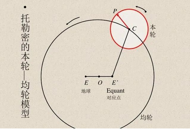
Ptolemy’s and Copernicus’s models are both unparalleled. If we want to make predictions through a “black box”, then Ptolemy’s geocentric model is superior. But if you want a simple model to “observe the model internally” (which is the starting point for explaining stellar motion theory), then Copernicus’s model is the best choice. Later, Kepler improved Copernicus’s model to elliptical orbits and proposed Kepler’s three laws of planetary motion, allowing Newton to explain planetary laws with a gravitational law applicable to Earth.
Therefore, it is important to note that the heliocentric model is not just a “black box” that provides predictions, but is given by several simple mathematical equations, although the “motion part” of the equations is minimal. Over the years, astronomy has been a source of inspiration for developing statistical techniques. Gauss and Legendre independently invented least squares regression around 1800 to predict the orbits of asteroids and other celestial bodies. In 1847, Cauchy invented the gradient descent method, also driven by astronomical predictions.
In physics, sometimes scholars can grasp all the details to find the “correct” theory, optimizing predictive accuracy and providing the best explanation for the data. These are all within the scope of viewpoints like Occam’s razor, which can be seen as a harmony between simplicity of assumptions, predictive capacity, and interpretability.
However, in many other fields, the relationship between the two goals of explanation and prediction is not so harmonious. If the goal is merely to predict observations, then a “black box” may be the best approach. On the other hand, if one wants explanatory information, such as causal models, general principles, or important features, then a model that can be understood and explained may be better the simpler it is.
The correct choice of model depends on its purpose. For example, consider a dataset of gene expression and phenotypes (such as certain diseases) containing many individuals. If the goal is to predict the likelihood of a person getting sick, then regardless of how complex it is or how many genes it depends on, the best predictive model adapted for that task should be used. In contrast, if the purpose is to identify some genes for further study, then the utility of a complex, very precise “black box” is limited.
Statistician Leo Breiman articulated this in his famous 2001 article on the two cultures of statistical modeling. The first is the “data modeling culture”, which focuses on simple generative models that can explain the data. The second is the “algorithmic modeling culture”, which is agnostic to how data is generated and focuses on finding models that can predict the data, regardless of how complex they are.
Article link: https://projecteuclid.org/journals/statistical-science/volume-16/issue-3/Statistical-Modeling–The-Two-Cultures-with-comments-and-a/10.1214/ss/1009213726.full
Breiman believed that statistics was overly dominated by the first culture, which caused two problems:
-
It led to irrelevant theories and questionable scientific conclusions.
-
It prevented statisticians from exploring exciting new problems.
Breiman’s paper sparked some controversy. Another statistician, Brad Efron, responded by saying that while he agreed with some points, he also emphasized that Breiman’s argument seemed to oppose frugality and scientific insight, supporting the labor-intensive creation of complex “black boxes”. However, in a recent article, Efron dismissed his earlier view, acknowledging that Breiman was more prescient, as “the focus of 21st-century statistics has largely evolved along the lines proposed by Breiman, centering on predictive algorithms”.
2. Classical vs. Modern Predictive Models
Machine learning, whether deep learning or not, has evolved along Breiman’s second viewpoint, focusing on prediction. This culture has a long history. For example, Duda and Hart’s textbook published in 1973 and Highleyman’s 1962 paper mentioned the content in the following figure, which is very easy for today’s deep learning researchers to understand:
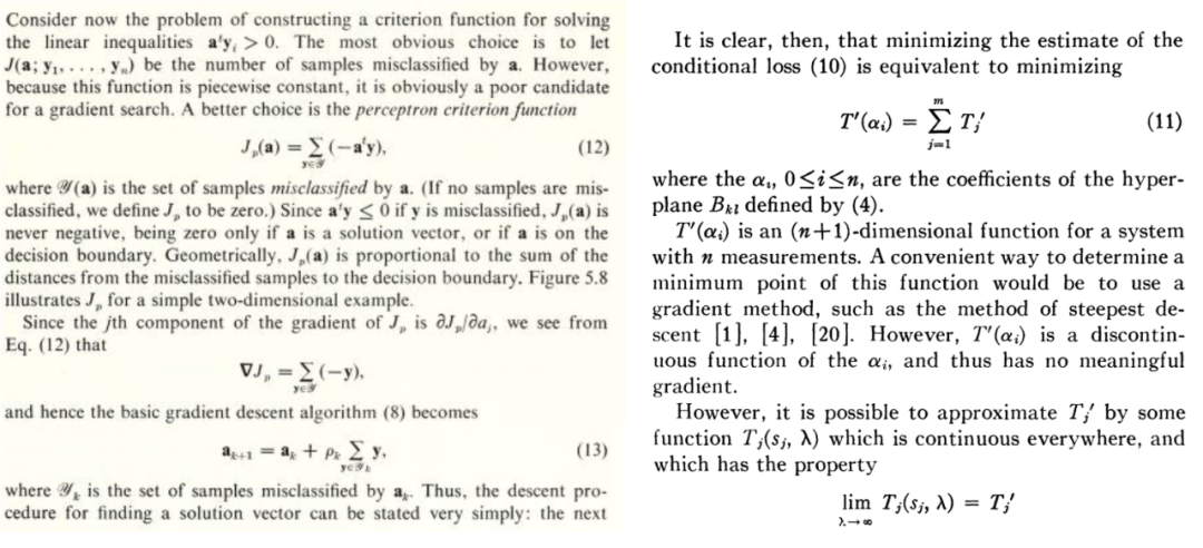
Excerpt from Duda and Hart’s textbook “Pattern Classification and Scene Analysis” and Highleyman’s 1962 paper “The Design and Analysis of Pattern Recognition Experiments”
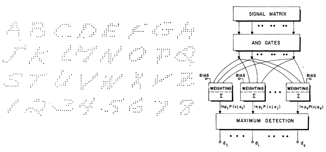
Similarly, the handwritten character dataset from Highleyman in the following figure and the architecture used to fit it (Chow, 1962) (accuracy about 58%) will resonate with many.
3. Why Is Deep Learning Different?
In 1992, Geman, Bienenstock, and Doursat wrote a pessimistic article about neural networks, arguing that “current feedforward neural networks are largely insufficient to solve the challenges of machine perception and machine learning.” Specifically, they believed that general neural networks would not succeed in handling difficult tasks, and their only path to success was through manually designed features. In their words: “Important attributes must be built-in or ‘hardwired’… rather than learned in any statistical sense.” In retrospect, Geman et al. were completely wrong, but it is more interesting to understand why they were wrong.
Deep learning is indeed different from other learning methods. Although deep learning may seem to be just about prediction, like nearest neighbors or random forests, it may have more complex parameters. This appears to be merely a quantitative difference rather than a qualitative one. However, in physics, once the scale changes by several orders of magnitude, it often requires an entirely different theory; the same is true for deep learning. The foundational processes of deep learning are completely different from classical models (whether parameterized or non-parameterized), even though their mathematical equations (and Python code) appear the same at a higher level.
To illustrate this, consider two different scenarios: fitting statistical models and teaching students mathematics.
Scenario A: Fitting a Statistical Model
The typical steps to fit a statistical model through data are as follows:
1. Here is some data (
( is
is the matrix;
 is
is the dimensional vector, which is the category label. Considering the data as coming from a structured model containing noise is the model to be fitted)
2. Use the above data to fit a model , and use an optimization algorithm to minimize empirical risk. This means finding such a
 that
that is minimized,
 representing the loss (indicating how close the predicted value is to the true value),
 is an optional regularization term.
3. The overall loss of the model should be minimized, that is, the generalization error should be relatively minimized.
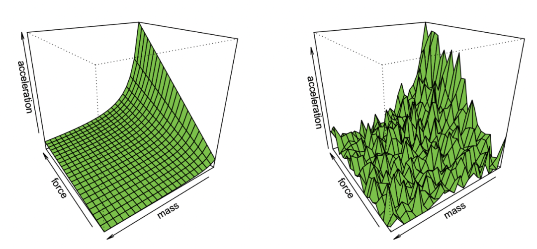
Effron’s demonstration of recovering Newton’s first law from observations containing noise
This very general example actually contains many elements, such as least squares linear regression, nearest neighbors, neural network training, etc. In classical statistical scenarios, we often encounter the following:
Trade-off: Suppose is the optimized model set (if the function is non-convex or contains regularization terms, careful selection of algorithms and regularization can yield model sets
 . The bias of the set
 is the closest approximation to the true value that can be achieved. The larger the set
 , the smaller the bias, and it may be 0 (if
 ).
).
However, as increases, the more samples are needed to narrow its member range, resulting in greater variance in the model output. The overall generalization error is the sum of bias and variance. Therefore, statistical learning is often a Bias-Variance trade-off, where the correct model complexity minimizes overall error. In fact, Geman et al. demonstrated their pessimistic attitude towards neural networks, asserting that the fundamental limitations posed by the Bias-Variance dilemma apply to all non-parametric inference models, including neural networks.
“The more the better” does not always hold: In statistical learning, more features or data do not necessarily improve performance. For example, learning from data containing many irrelevant features is quite challenging. Similarly, learning from a mixture model, where data comes from one of two distributions (e.g., and
and ), is more difficult than learning each distribution independently.
Diminishing returns: In many cases, the number of data points required to reduce predictive noise to the level is related to the parameters
 and
and ; that is, the number of data points is approximately equal to
 . In this case, about k samples are needed to initiate, but once this is done, diminishing returns occur; that is, if it takes
 points to achieve 90% accuracy, then about an additional
 points are needed to raise the accuracy to 95%. Generally, as resources increase (whether data, model complexity, or computation), people expect to achieve finer distinctions rather than unlocking specific new features.
Severe dependence on loss and data: When fitting models to high-dimensional data, any small detail can make a significant difference. Choices like L1 or L2 regularizers are crucial, not to mention using completely different datasets. Different numbers of high-dimensional optimizers can also differ significantly from each other.
Data is relatively “pure”: It is often assumed that data is sampled independently from some distribution. While points close to the decision boundary are hard to classify, considering the concentration phenomenon measured in high dimensions, most points can be considered close in distance. Therefore, in classical data distributions, the distance differences between data points are not significant. However, mixture models can show this difference, and thus, unlike other issues mentioned above, this difference is common in statistics.
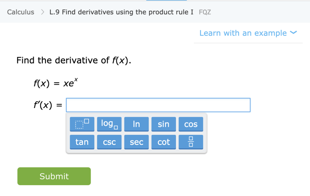
Scenario B: Learning Mathematics
In this scenario, we assume you want to teach students mathematics (such as calculating derivatives) through some instructions and exercises. This scenario, while not formally defined, has some qualitative characteristics:
Learning a skill rather than approximating a statistical distribution: In this case, students are learning a skill rather than estimating/predicting some quantity. Specifically, even if the mapping of exercises to the function of solutions cannot be used as a “black box” to solve some unknown tasks, the thought patterns formed by students when solving these problems are still useful for unknown tasks.
The more the better: Generally, students who solve more problems and cover a wider range of problem types perform better. Simultaneously doing some calculus problems and algebra problems does not lead to a decline in students’ calculus performance; on the contrary, it may help improve their calculus scores.
From skill enhancement to automated representation: While in some cases, the rewards for solving problems may also diminish, students’ learning goes through several stages. There is a stage where solving some problems helps understand concepts and unlock new abilities. Furthermore, when students repeatedly encounter a specific type of problem, they will form an automated problem-solving process for similar problems, transitioning from previous skill enhancement to automated problem-solving.
Performance independent of data and loss: There are multiple methods to teach mathematical concepts. Students learning through different books, educational methods, or grading systems can ultimately learn the same content and develop similar mathematical abilities.
Some problems are more difficult: In mathematics practice, we often see a strong correlation between how different students solve the same problem. For a problem, there seems to be an inherent difficulty level and a natural progression of difficulty that is most beneficial for learning.
4. Is Deep Learning More Like Statistical Estimation or Student Skill Learning?
Which of the above two scenarios is more appropriate to describe modern deep learning? Specifically, what is the reason for its success? Statistical model fitting can be well expressed using mathematics and code. In fact, a standard Pytorch training loop trains deep networks through empirical risk minimization:
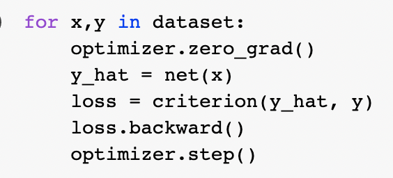
On a deeper level, the relationship between these two scenarios is not clear. To be more specific, here is an example of a specific learning task. Consider a classification algorithm trained using the “self-supervised learning + linear probing” method. The specific algorithm is trained as follows:
1. Assume the data is a sequence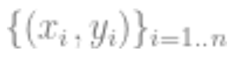 , where
 is a data point (such as an image),
 is the label.
2. First obtain the representation function of the deep neural network. By minimizing some type of self-supervised loss function, train this function using only data points
 without using labels. Examples of such loss functions include reconstruction (recovering input from other inputs) or contrastive learning (the core idea is to contrast positive and negative samples in feature space, learning the feature representation of samples).
3. Use the fully labeled data to fit a linear classifier
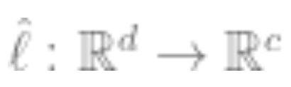 (
( is the number of classes), to minimize cross-entropy loss. Our final classifier is:
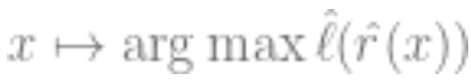
Step 3 applies only to linear classifiers, so the “magic” occurs in step 2 (self-supervised learning of deep networks). Some important properties of self-supervised learning include:
Learning a skill rather than approximating a function: Self-supervised learning is not about approximating functions; it is about learning representations that can be used for various downstream tasks (this is the dominant paradigm in natural language processing). Obtaining downstream tasks through linear probing, fine-tuning, or incentives is secondary.
The more the better: In self-supervised learning, the quality of representations improves with the increase in data quantity, and does not worsen by mixing data from several sources. In fact, the more diverse the data, the better.

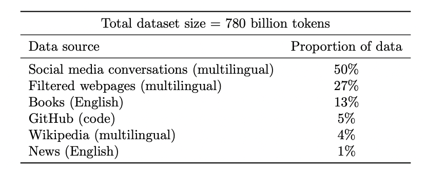
Google PaLM model’s dataset
Unlocking new abilities: As resources (data, computation, model size) are invested, deep learning models also improve discontinuously. This has been demonstrated in some combined environments.
As the model scale increases, PaLM shows discontinuous improvements in benchmarks and unlocks surprising capabilities, such as explaining why jokes are funny.
Performance is almost independent of loss or data: There are multiple self-supervised losses; in image research, various contrastive and reconstruction losses are actually used, while language models use unidirectional reconstruction (predicting the next token) or mask models, predicting masked inputs from left and right tokens. Slightly different datasets can also be used. These may affect efficiency, but as long as “reasonable” choices are made, the original resources typically enhance predictive performance more than the specific loss or dataset used.
Some situations are more difficult than others: This is not specific to self-supervised learning. Data points seem to have some inherent “difficulty levels”. In fact, different learning algorithms have different “skill levels”, and different data points have different “difficulty levels” (the probability of a classifier correctly classifying points
 increases monotonically with skill, while decreasing monotonically with difficulty).
The “skill vs. difficulty” paradigm is the clearest explanation for the “accuracy on the line” phenomenon discovered by Recht et al. and Miller et al. Papers by Kaplen, Ghosh, Garg, and Nakkiran also demonstrate that different inputs in the dataset have inherent “difficulty profiles”, which are typically robust across different model families.
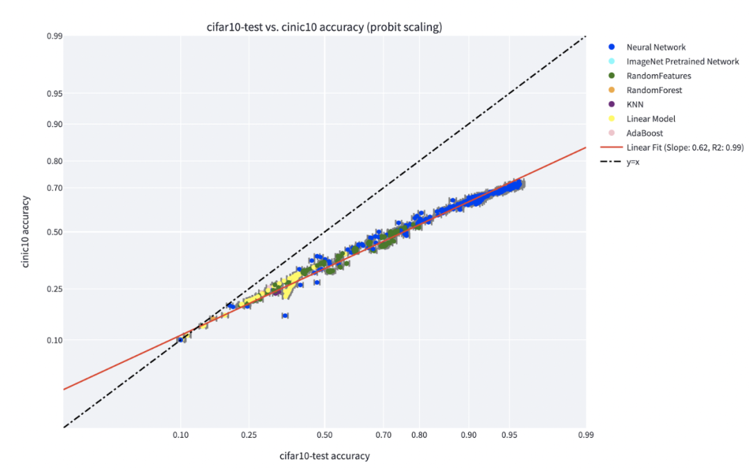
The top figure describes the probabilities of the most likely categories as a function of the global accuracy of a classifier for a specific category, indexed by training time. The bottom pie chart shows the different datasets decomposed into different types of points (note that this decomposition is similar for different neural structures).
Training is teaching: The training of modern large models seems more like teaching students rather than fitting the model to data. When students do not understand or feel tired, they “rest” or try different methods (training variations). Meta’s large model training logs are enlightening—besides hardware issues, we can also see interventions, such as switching different optimization algorithms during training, or even considering “hot swapping” activation functions (GELU to RELU). If model training is viewed as fitting data rather than learning representations, then the latter does not make much sense.
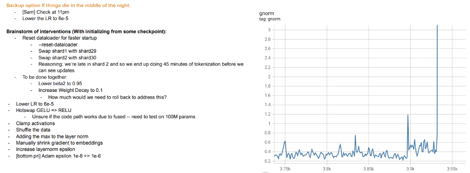
Excerpt from Meta’s training log
4.1) What About Supervised Learning?
We previously discussed self-supervised learning, but a typical example of deep learning remains supervised learning. After all, deep learning’s “ImageNet moment” came from ImageNet. So does what has been discussed still apply in this setting?
First, the emergence of large-scale supervised deep learning is somewhat coincidental, thanks to the availability of large, high-quality labeled datasets (i.e., ImageNet). If you have a vivid imagination, you could envision an alternative history where deep learning first made breakthroughs through unsupervised learning in natural language processing before transitioning to vision and supervised learning.
Second, there is evidence that, despite using completely different loss functions, supervised learning and self-supervised learning behave similarly “internally”. Both typically achieve the same performance. Specifically, for each , one can combine the first k layers of a deep model trained through self-supervision with the last d-k layers of a supervised model, with minimal performance loss.
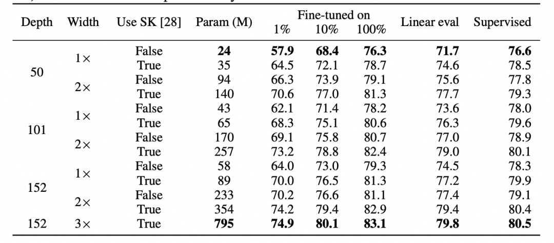
Table from the SimCLR v2 paper. Note the general similarity in performance between supervised learning, fine-tuning (100%), self-supervised, and self-supervised + linear probing (source: https://arxiv.org/abs/2006.10029)
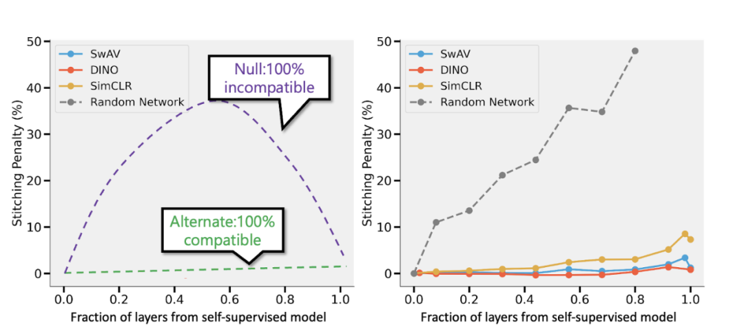
Results of stitching together self-supervised models and supervised models by Bansal et al. (https://arxiv.org/abs/2106.07682). Left: If the accuracy of the self-supervised model (e.g.,) is 3% lower than that of the supervised model, then when the p part of the layer comes from the self-supervised model, the fully compatible representation will lead to a stitching penalty of p 3%. If the models are entirely incompatible, we expect accuracy to drop sharply as more models are merged. Right: Actual results of merging different self-supervised models.
The advantage of self-supervised + simple models is that they can separate feature learning or “deep learning magic” (accomplished by deep representation functions) from statistical model fitting (performed by linear or other “simple” classifiers on top of this representation).
Finally, although this is more speculative, it seems that “meta-learning” often equates to learning representations (see: https://arxiv.org/abs/1909.09157, https://arxiv.org/abs/2206.03271 ), which can be seen as further evidence that this is largely what is going on, regardless of the optimization objectives of the models.
4.2) What About Over-Parameterization?
This article skips typical examples where it is believed that statistical learning models and deep learning differ in practice: the lack of “Bias-Variance trade-off” and the good generalization ability of over-parameterized models.
Why skip this? There are two reasons:
-
First, if supervised learning is indeed equal to self-supervised + simple learning, then this may explain its generalization ability.
-
Second, over-parameterization is not the key to deep learning’s success. Deep networks are special not because they are large relative to the number of samples, but because they are large in absolute terms. In fact, even for very large language models, their datasets are larger.
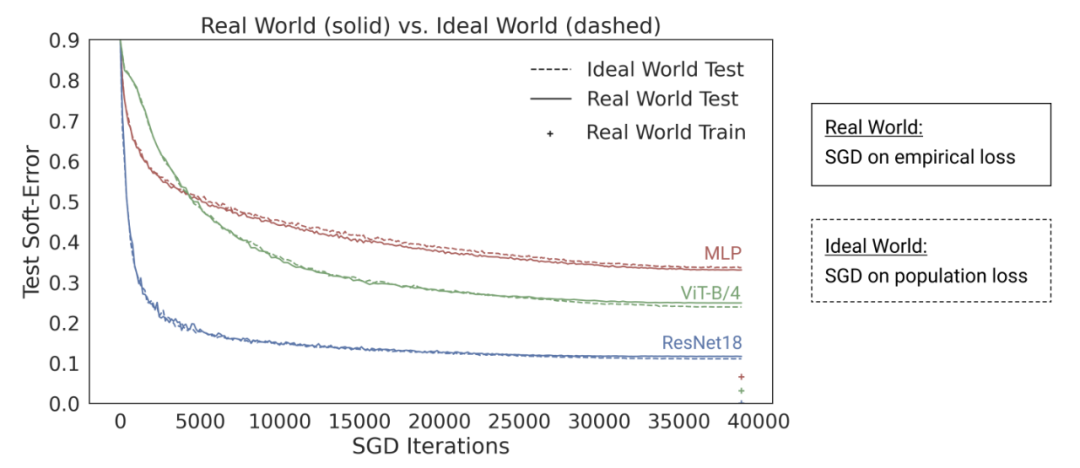
Nakkiran-Neyshabur-Sadghi’s “deep bootstrap” paper suggests that modern architectures behave similarly in both “over-parameterized” or “under-sampled” states (the model trains multiple epochs on limited data until overfitting: “Real World” in the above image), as well as in “under-parameterized” or “online” states (the model trains for a single epoch, seeing each sample only once: “Ideal World” in the above image). Source: https://arxiv.org/abs/2010.08127
Conclusion
Statistical learning certainly plays a role in deep learning. However, viewing deep learning simply as fitting a model with more parameters than classical models, despite using similar terms and code, overlooks many aspects that are crucial to its success. The metaphor of teaching students mathematics is not perfect either.
Like biological evolution, although deep learning contains many reused rules (such as gradient descent of empirical loss), it produces highly complex results. It seems that at different times, different components of the network learn different things, including representation learning, predictive fitting, implicit regularization, and pure noise. Researchers are still searching for suitable perspectives to pose questions about deep learning, let alone answer them.
Original link: https://windowsontheory.org/2022/06/20/the-uneasy-relationship-between-deep-learning-and-classical-statistics/
Editor: Huang Jiyan