Notes from Andrew Ng’s DeepLearning.ai Course
[Andrew Ng’s DeepLearning.ai Notes 1] Intuitive Explanation of Logistic Regression
[Andrew Ng’s DeepLearning.ai Notes 2] Simple Explanation of Neural Networks (Part 1)
[Andrew Ng’s DeepLearning.ai Notes 2] Simple Explanation of Neural Networks (Part 2)
Is deep learning not working well? Andrew Ng will help you optimize neural networks (1)
[deeplearning.ai] Deep Learning: Optimizing Neural Networks (2)
When building a machine learning system and achieving some initial results, substantial improvements are often needed to obtain the most satisfactory outcomes. As previously discussed in optimizing neural networks, there are various methods for improvement, which may include collecting more data, applying regularization, or using different optimization algorithms.
To pinpoint the direction for improvement and make a machine learning system work faster and more effectively, it is essential to learn some strategies commonly used in building machine learning systems.
1. Orthogonalization
One of the challenges in building a machine learning system is the multitude of aspects that can be tried or changed. For instance, there are many hyperparameters that need to be tuned. It is crucial to grasp the direction of trials and changes and recognize the impact of each adjustment made.
Orthogonalization is a system design property that ensures modifying an algorithm instruction or component in a system does not produce or propagate side effects to other components in the system.
It makes it easier to validate one algorithm independently of another while also reducing design and development time.
For example, when learning to drive a car, you mainly learn the three basic control methods: steering, accelerating, and braking. These three controls do not interfere with each other; you just need to practice repeatedly to master them.
However, if you had to learn to drive a car with only one joystick that controls a certain steering angle and speed with each operation, the learning cost would increase significantly. This is the essence of orthogonalization.
When designing a supervised learning system, the following four assumptions must be satisfied, and they should be orthogonal:
-
The model built performs well on the training set;
-
The model built performs well on the development set (validation set);
-
The model built performs well on the test set;
-
The model built performs well in real-world applications.
Once orthogonalization is achieved, if you find:
-
Poor performance on the training set — try deeper neural networks or different optimization algorithms;
-
Poor performance on the development set — try regularization or adding more training data;
-
Poor performance on the test set — try using more development data for validation;
-
Poor performance in real applications — this may be due to incorrect test set configuration or cost function evaluation errors.
Faced with various issues, orthogonalization can help us more accurately locate and effectively solve problems.
2. Single-Number Evaluation
When constructing a machine learning system, setting a single-number evaluation metric allows for a quicker determination of which results are better after several adjustments.
For a classifier, the performance metric is usually the classification accuracy, which is the ratio of correctly classified samples to the total number of samples. This can serve as a single-number evaluation metric. For example, several algorithms for the previous cat classifier were evaluated based on accuracy.
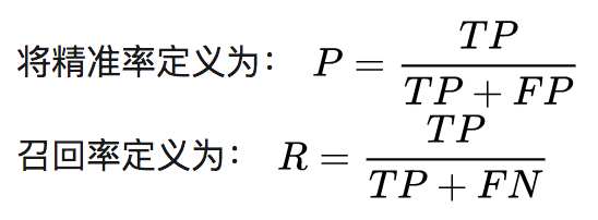
Common evaluation metrics for binary classification problems include precision and recall, considering the class of interest as the positive class and all others as the negative class. The correct and incorrect predictions made by the classifier can be represented as:
-
TP (True Positive) — number of true positives predicted
-
FN (False Negative) — number of false negatives predicted
-
FP (False Positive) — number of false positives predicted
-
TN (True Negative) — number of true negatives predicted

When faced with situations that are difficult to judge, the F1 score is needed to evaluate the performance of two classifiers.

The F1 score is defined as:
The F1 score is actually the harmonic mean of precision and recall, which is a method that improves upon the average value, yielding better results than simply taking the average.
Thus, the F1 score for classifier A is calculated to be 92.4%, while for classifier B it is 91.0%, indicating that classifier A performs better. Here, the F1 score serves as the single-number evaluation metric.
3. Satisficing and Optimizing Metrics

However, sometimes the evaluation criteria are not limited to a single-number evaluation metric. For instance, in the case of several cat classifiers, one might want to consider both their recognition accuracy and runtime. However, combining these two metrics into a single-number evaluation metric may not be sufficient.
In this case, one metric needs to be set as the optimizing metric, while others are treated as satisficing metrics.
In the earlier example, accuracy serves as an optimizing metric since the goal is to classify correctly as much as possible, while runtime serves as a satisficing metric. If you want the classifier’s runtime to not exceed a certain value, you should select the classifier with the highest accuracy within that limit, thereby making a trade-off.
In addition to using these criteria to evaluate a model, one must also learn to adjust evaluation metrics when necessary, or even change training data.
For example, if two cat classifiers A and B have recognition errors of 3% and 5% respectively, but due to some reasons, classifier A misclassifies adult content as cats, causing user discomfort, while B does not produce such issues, then classifier B, despite having a higher recognition error, is the better classifier. The following formula can be used to calculate the error recognition rate:

Additionally, a weight ω(i) can be set such that when x(i) is adult content, ω(i) is 10, otherwise it is 1, to differentiate between adult content and other misclassified images:

Therefore, it is essential to determine an evaluation metric based on actual conditions to ensure its optimality.
4. Data Processing
When building a machine learning system, the method of processing the dataset will affect the progress of the entire construction process. As previously noted, the collected existing data is generally divided into training set, development set, and test set, with the development set also referred to as the cross-validation set.
In constructing a machine learning system, different methods should be used to train various models on the training set, and then use the development set to evaluate the model’s performance. Once a model is deemed sufficiently good, it is then tested with the test set.
First, it is important to note that the sources of the development set and test set should be the same and must be randomly sampled from all data. The selected development and test sets should also be as consistent as possible with the real data the machine learning system will face to avoid straying from the target.
Secondly, attention should be paid to the size distribution of each dataset. In the early days of machine learning, typically 70% of the total dataset was used as the training set, and the remaining 30% as the test set; or if a development set was included, 60% was used for training, with 20% each for development and testing.
This division was reasonable when the amount of data obtained was small. However, in today’s era of machine learning, where data is typically in the thousands or millions, traditional data division methods should not be strictly followed.
If one obtains one million data samples, using 98% of the data as the training set, and only 1%, or ten thousand data points, as the development and test sets is sufficient.
Thus, data division should be based on actual circumstances rather than rigidly adhering to tradition.
The size of the test set should be set sufficiently to improve the credibility of the overall system performance, and the size of the development set should also be adequate for evaluating several different models.
5. Comparing Human Performance Levels
Today, designing and establishing a machine learning system has become simpler and more efficient than before. Some machine learning algorithms can now perform at levels comparable to humans in many fields, such as the globally renowned AlphaGo developed by Google DeepMind.
However, many tasks can be performed nearly perfectly by humans, and machine learning systems are attempting to reach or even exceed human performance levels.

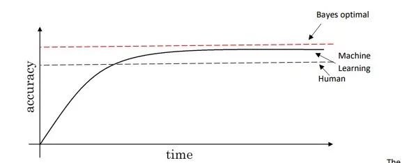
The image above shows the changes in machine learning and human performance levels over time. Generally, when machine learning surpasses human performance levels, its progress slows down significantly. One important reason for this is that humans perform at levels close to Bayes Error on certain natural perception problems.
Bayes Error is defined as the optimal possible error, in other words, no mapping function from x to accuracy y can exceed this value.
When the performance of the established machine learning model has not yet reached human performance levels, various means can be employed to enhance it. For example, training with manually labeled data, understanding why humans can correctly identify through manual error analysis, or conducting variance and bias analysis.
The concepts of bias and variance were previously discussed in optimizing neural networks. By comparing a machine learning model’s performance to human performance on a particular task, one can clearly indicate the model’s performance level, thus determining whether to focus on reducing bias or variance in subsequent work.

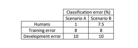
The difference between the training set error and the human performance error is called avoidable bias.
For example, in the two scenarios depicted, comparing the error rates of humans and machine learning models shows that in scenario A, the learning algorithm’s error rate has a significant avoidable bias compared to human error rates. In this case, subsequent work should focus on reducing the training set error rate to decrease bias. In scenario B, the learning algorithm performs comparably to humans, with an avoidable bias of only 0.5%, so the focus should shift to minimizing the variance in the development and training sets.
Human performance levels provide an estimate of Bayes error, when training a machine learning system for a certain task, using human performance levels as Bayes error avoids optimizing the training error rate directly to 0% during training.
Therefore, when obtaining human error data for a task, this data can be used as a proxy for Bayes error to analyze the bias and variance of the learning algorithm.
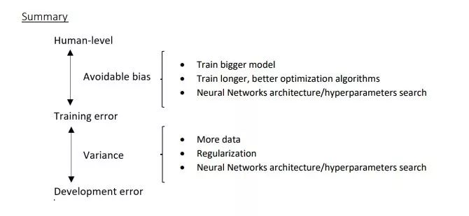
If the error difference between the training set and human performance levels is greater than the difference between the training set and development set, future efforts should focus on reducing bias; conversely, if it is less, efforts should focus on reducing variance.

The image above summarizes various methods for addressing bias and variance. In summary, a small avoidable bias indicates that the model’s training process is well executed; an acceptable range of variance means that the model performs similarly on the development and test sets as it does on the training set.
Additionally, if an avoidable error is negative, meaning the machine learning model’s performance exceeds human performance levels (the proxy for Bayes error), this does not imply that the model’s performance has reached its peak. To further enhance its performance, alternative optimization methods must be sought.
Currently, machine learning has achieved this in many fields, such as online advertising, product promotion, predicting logistics transport times, credit assessment, and more.
Note:All images and materials referenced in this article are compiled and translated from Andrew Ng’s Deep Learning series courses, with all rights reserved. The translation and compilation quality may be limited; please feel free to point out any inaccuracies.

Recommended Reading:
Markov Decision Processes: Markov Processes
[Deep Learning Practice] How to Handle Variable-Length Sequences in RNNs with PyTorch
[Fundamental Theories of Machine Learning] Detailed Explanation of Maximum A Posteriori Probability Estimation (MAP)
Welcome to follow our public account for learning and communication~

