Source: Machine Learning Algorithms

This article is about 5000 words long, and it is recommended to read in 8 minutes
This article summarizes some basic concepts about Convolutional Neural Networks (CNN).
This article summarizes some basic concepts about Convolutional Neural Networks (CNN) and provides detailed explanations of the principles involved. Through this article, one can gain a comprehensive understanding of Convolutional Neural Networks (CNN), making it very suitable as an introductory learning resource for Deep Learning. Below is the full content of this blog!
1. What is a Convolutional Neural Network?
The concept of Convolutional Neural Networks (Convolutional Neural Networks, CNN) can be traced back to the 1980s and 1990s, but there was a period when this concept was “shelved” due to the relatively backward hardware and software technology at that time. With the emergence of various deep learning theories and the rapid development of numerical computing devices, Convolutional Neural Networks have developed rapidly.
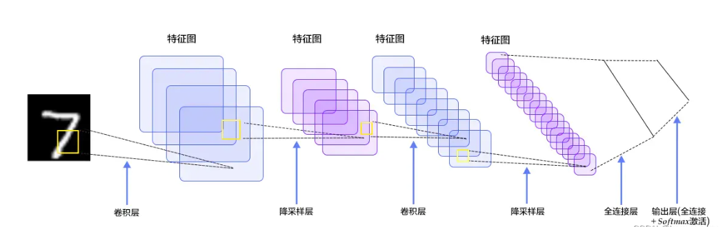
So what exactly is a Convolutional Neural Network? Taking handwritten digit recognition as an example, the entire recognition process is as follows:
Figure 1: Handwritten Digit Recognition Process
The above process is the entire process of recognizing handwritten digits. I have previously written related blogs on this project and open-sourced the code. Interested readers can refer to:
https://blog.csdn.net/IronmanJay/article/details/128434368?spm=1001.2014.3001.5501
That said, the entire process requires calculations at the following layers:
-
Input Layer: Input image and other information
-
Convolutional Layer: Used to extract the low-level features of the image
-
Pooling Layer: Prevents overfitting and reduces the dimensionality of the data
-
Fully Connected Layer: Summarizes the low-level features and information of the image obtained from the convolutional and pooling layers
-
Output Layer: Obtains the result with the highest probability based on the information from the fully connected layer
It can be seen that the most important layer is the convolutional layer, which is also the origin of the name Convolutional Neural Network. Below, the relevant content of these layers will be explained in detail.
The input layer is quite simple; its main task is to input image and other information since Convolutional Neural Networks primarily deal with image-related content. However, is the image we see with our eyes the same as the image processed by a computer?
Clearly, they are not the same. For the input image, it must first be converted into the corresponding two-dimensional matrix. This two-dimensional matrix is composed of the pixel values of each pixel in the image. We can look at an example, as shown in the image below of the handwritten digit “8,” which is stored as a two-dimensional matrix composed of pixel values after being read by the computer.
Figure 2: Grayscale Image of the Digit 8 and Its Corresponding Two-Dimensional Matrix
The above image is also called a grayscale image because the range of each pixel value is from 0 to 255 (from pure black to pure white), indicating the intensity of its color. There are also black and white images where each pixel value is either 0 (indicating pure black) or 255 (indicating pure white).
The most common in our daily life is the RGB image, which has three channels: red, green, and blue. The range of each pixel value in each channel is also from 0 to 255, indicating the intensity of the color of each pixel.
However, we usually process mostly grayscale images because they are easier to handle (smaller value range, simpler colors). Some RGB images are also converted into grayscale images before being input into the neural network for easier computation; otherwise, handling three channels together would result in a very large computational load.
Of course, with the rapid development of computer performance, some neural networks can now also process three-channel RGB images.
Now we know that the role of the input layer is to convert the image into its corresponding two-dimensional matrix composed of pixel values and to store this two-dimensional matrix, waiting for operations from the subsequent layers.
So how should the image be processed after it is inputted?
Assuming we have obtained the two-dimensional matrix of the image and want to extract features from it, the convolution operation will assign a high value to areas where features exist; otherwise, it will assign a low value. This process needs to calculate the product value with the Convolution Kernel.
Suppose our input image is a person’s head, and the person’s eyes are the features we want to extract. We will use the person’s eyes as the convolution kernel and move it across the person’s head image to determine where the eyes are, as shown in the following process:
Figure 3: Process of Extracting the Feature of a Person’s Eyes
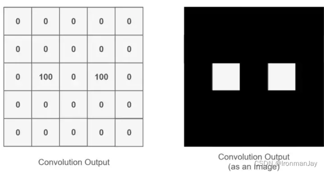
Through the entire convolution process, we obtain a new two-dimensional matrix, which is also known as the Feature Map. Finally, we can color the obtained Feature Map (I am just using an analogy, for example, high values as white and low values as black), and we can extract features about the person’s eyes, as shown below:
Figure 4: Result of Extracting the Feature of a Person’s Eyes
Looking at the description above may seem a bit confusing; don’t worry. First, the convolution kernel is also a two-dimensional matrix, but this two-dimensional matrix must be smaller or equal to the two-dimensional matrix of the input image. The convolution kernel moves across the two-dimensional matrix of the input image, computing the sum of the products at each position, as shown in the following diagram:
Figure 5: The Convolution Process
As can be seen, the entire process is a dimensionality reduction process. By continuously moving the convolution kernel and calculating, we can extract the most useful features from the image.
We usually refer to the new two-dimensional matrix obtained from the convolution kernel calculation as the Feature Map. For example, in the animated diagram above, the dark blue square moving below is the convolution kernel, while the cyan square above is the Feature Map.
Some readers may notice that every time the convolution kernel moves, the middle position is calculated multiple times, while the edges of the input image’s two-dimensional matrix are only calculated once. Will this lead to inaccurate calculation results?
Let’s think carefully. If the edges are calculated only once while the middle is calculated multiple times, the obtained Feature Map will also lose edge features, ultimately leading to inaccurate feature extraction. To solve this problem, we can expand one or more circles around the original two-dimensional matrix of the input image so that every position can be fairly computed, thus not losing any features. This process can be seen in the following two cases. This method of solving feature loss by expanding is called Padding.
• Padding value is 1, expanding one circle
Figure 6: Convolution Process with Padding of 1
• Padding value is 2, expanding two circles
Figure 7: Convolution Process with Padding of 2
Now, what if the situation is a bit more complicated? If we use two convolution kernels to extract features from a color image?
As previously mentioned, color images have three channels, meaning a color image will have three two-dimensional matrices. Of course, we will only consider the first channel for demonstration purposes, as it would be too complicated otherwise.
At this time, we use two sets of convolution kernels, each set of convolution kernels is used to extract features from the two-dimensional matrix of its own channel. As mentioned, we will only consider the first channel, so we only need to use the first convolution kernel from each set of convolution kernels to calculate the Feature Map, as shown in the following process:
Figure 8: Convolution Process with Two Convolution Kernels
Looking at the animated diagram above may seem a bit bewildering. Let me explain. According to the previous logic, the input image is a color image with three channels, so the size of the input image is 7×7×3. Since we are only considering the first channel, we are extracting features from the first 7×7 two-dimensional matrix.
We only need to use the first convolution kernel from each set of convolution kernels, and here some readers may notice the Bias, which is the bias term. The final calculation result is added to it, and ultimately we can obtain the Feature Map through calculations.
It can be observed that the number of Feature Maps corresponds to the number of convolution kernels used. Since we are only using two convolution kernels, we will obtain two Feature Maps.
That concludes the relevant knowledge about the convolutional layer. Of course, this article is just an introduction, so there are some more complex content not discussed in depth, which will require further study and summarization later.
As we mentioned earlier, the number of convolution kernels corresponds to the number of Feature Maps. In reality, the situation is certainly more complex, leading to many convolution kernels and consequently more Feature Maps. When there are many Feature Maps, it means we have obtained many features, but are all these features necessary?
Clearly not; in fact, there are many features that we do not need, and these redundant features usually lead to the following two problems:
To solve this problem, we can utilize the pooling layer. So what is a pooling layer?
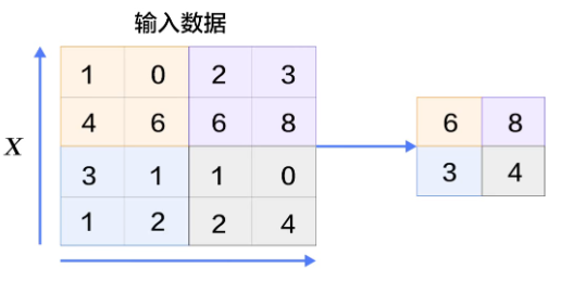
The pooling layer, also known as down-sampling, means that after performing convolution operations, we extract the most representative features from the obtained Feature Maps, which can help reduce overfitting and lower dimensionality. This process is as follows:
Figure 9: The Pooling Process
Some readers may ask what rules should be used for feature extraction?
This process is similar to the convolution process, where a small square moves across the image, and each time we take the most representative feature from this square area. But how do we extract the most representative feature? There are usually two methods:
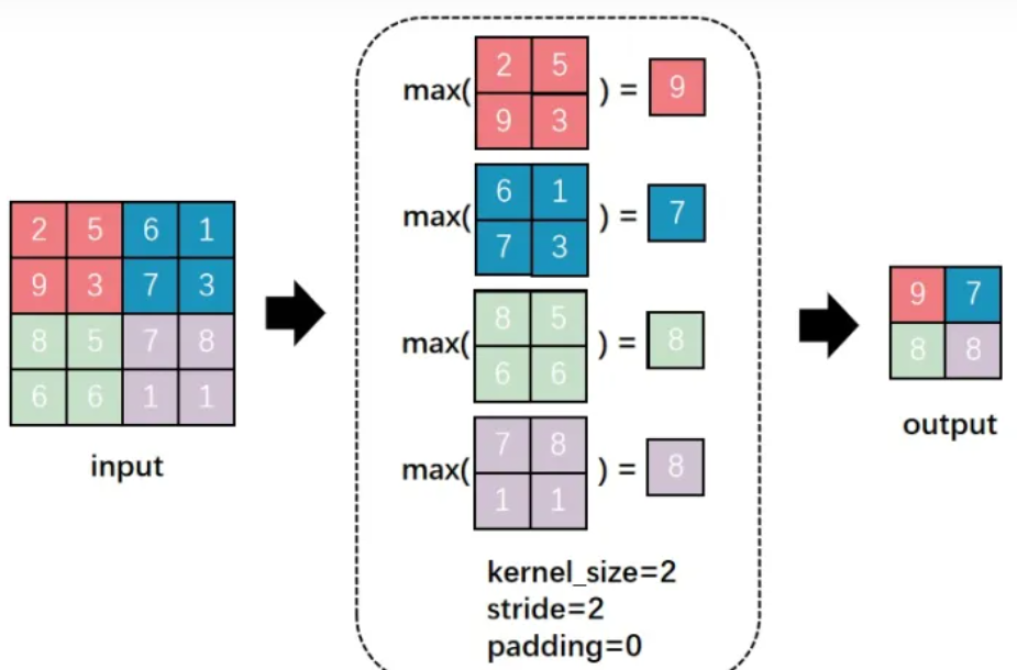
As the name suggests, max pooling involves taking the maximum value from all values in the square, which represents the most representative feature at that position. This process is as follows:
Figure 10: The Max Pooling Process
Here are a few parameters that need to be explained:
① kernel_size = 2: The square size used in the pooling process is 2×2. If it were in the convolution process, it would mean the convolution kernel size is 2×2.
② stride = 2: Each time the square moves two positions (from left to right, from top to bottom), this process is actually similar to the convolution operation process.
③ padding = 0: This has been introduced before; if this value is 0, it means no expansion has been performed.
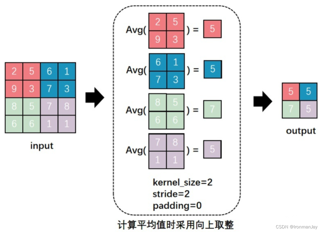
Average pooling means taking the average of all values in this square area, considering the impact of each position’s value on this feature. The average pooling calculation is also quite simple, as shown in the following diagram:
Figure 11: The Average Pooling Process
The meanings of the parameters are consistent with those explained for max pooling. Additionally, it should be noted that when calculating average pooling, rounding up is used.
The above describes all operations of the pooling layer. Let’s review: after pooling, we can extract more representative features.
At the same time, it reduces unnecessary computations, which greatly benefits neural network calculations in reality, as neural networks are very large in real situations. After the pooling layer, model efficiency can be significantly improved.
Therefore, the pooling layer has many advantages, which can be summarized as follows:
-
It retains the original features of the original image while reducing the number of parameters.
-
Effectively prevents overfitting.
-
Brings translation invariance to Convolutional Neural Networks.
We have already introduced the first two advantages; so what is translation invariance? It can be illustrated with one of our previous examples, as shown in the following image:
Figure 12: Translation Invariance of Pooling
As can be seen, the positions of the two original images are different; one is normal, while the other has the person’s head slightly shifted to the left.
After the convolution operation, the corresponding Feature Maps are obtained for each original image. The positions of the eye features in the two Feature Maps correspond to the positions of the original images. One eye feature’s position is normal, while the other is slightly shifted.
While humans can distinguish this, neural network calculations may introduce errors, as the expected position of the eye feature may not appear. What should we do?
At this point, using the pooling layer for pooling operations reveals that although the eye features in the two images are not at the same position before pooling, after pooling, the positions of the eye features are the same. This brings convenience to subsequent neural network calculations. This property is called the translation invariance of pooling.
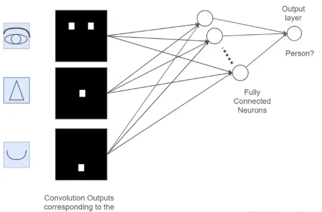
Assuming we have the example of the person’s head again, now that we have extracted the features of the person’s eyes, nose, and mouth through convolution and pooling, how can we use these features to determine whether the image is of a person’s head?
At this point, we only need to “flatten” all the extracted Feature Maps, changing their dimensions to 1 × x 1×x1×x. This process is known as the fully connected process.
In other words, in this step, we expand all the features and perform calculations, ultimately obtaining a probability value. This probability value indicates the likelihood that the input image is of a person’s head, as shown in the following process:
Figure 13: The Fully Connected Process
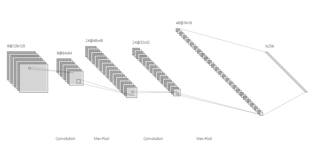
Looking at this process alone may still not be very clear, so we can combine the previous processes with the fully connected layer, as shown in the following diagram:
Figure 14: The Entire Process
It can be seen that after two rounds of convolution and max pooling, we obtain the final Feature Map. The features at this point are calculated, making them highly representative. Finally, through the fully connected layer, we expand them into a one-dimensional vector and perform one last calculation to obtain the final recognition probability. This is the entire process of a Convolutional Neural Network.
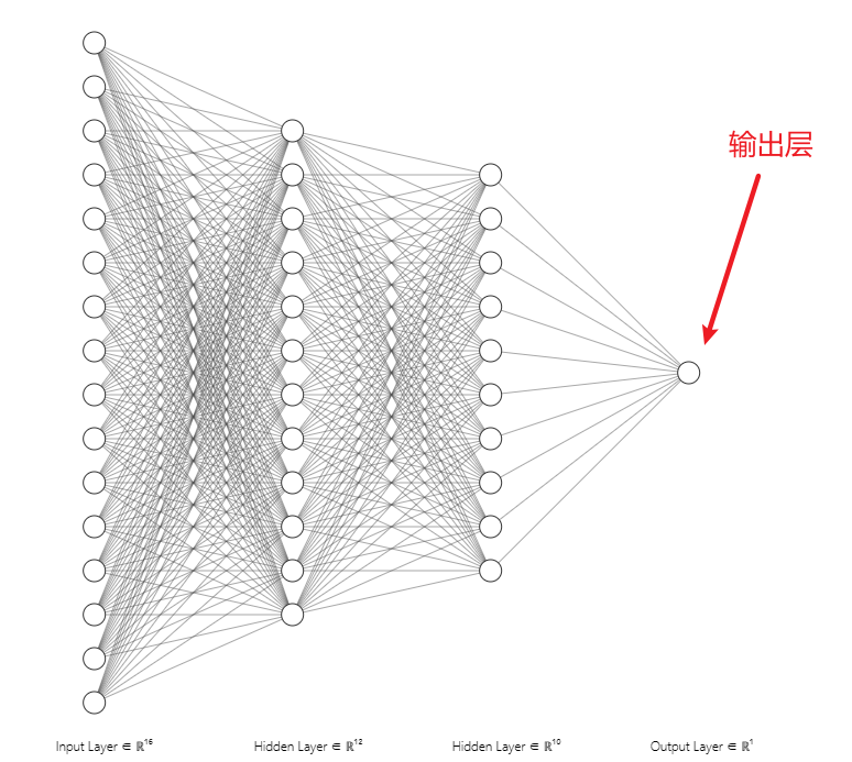
The output layer of a Convolutional Neural Network is relatively straightforward to understand. We simply need to calculate the recognition value’s probability from the one-dimensional vector obtained from the fully connected layer. Of course, this calculation can be linear or nonlinear.
In deep learning, the results we need to recognize are generally multi-class, so each position will have a probability value representing the likelihood of being recognized as the current value. The maximum probability value is taken as the final recognition result.
During training, we can continuously adjust parameter values to make the recognition results more accurate, thereby achieving the highest model accuracy.
Figure 15: Output Layer Diagram
7. Review of the Entire Process
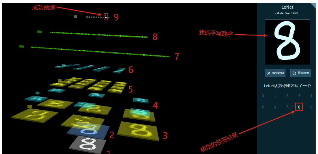
The most classic application of Convolutional Neural Networks is perhaps handwritten digit recognition. For example, if I now write a number 8, how does the Convolutional Neural Network recognize it? The entire recognition process is shown in the diagram below:
Figure 16: The Process of Handwritten Digit Recognition
1. Convert the handwritten digit image into a pixel matrix
2. Perform convolution operations on the pixel matrix with non-zero padding to preserve edge features and generate a Feature Map
3. Perform convolution operations with six convolution kernels on this Feature Map, resulting in six Feature Maps
4. Perform pooling operations (also known as down-sampling operations) on each Feature Map, retaining features while reducing data flow, generating six small images. These six small images resemble the previous layer’s Feature Maps but are smaller in size.
5. Perform a second convolution operation on the six small images obtained after pooling, generating more Feature Maps
6. Perform pooling operations (down-sampling operations) on the Feature Maps generated from the second convolution
7. Perform the first fully connected operation on the features obtained after the second pooling
8. Perform the second fully connected operation on the results of the first fully connected operation
9. Perform the final operation on the results of the second fully connected operation. This operation can be linear or nonlinear. Ultimately, each position (a total of ten positions, from 0 to 9) will have a probability value representing the likelihood of recognizing the input handwritten digit as the corresponding digit. The value of the position with the highest probability is taken as the recognition result.
As can be seen, the upper right is my handwritten digit, and the lower right is the model (LeNet) recognition result. The final recognition result is consistent with my input handwritten digit, as can be seen from the top left of the image, indicating that this model can successfully recognize handwritten digits.
This concludes the entire content of this blog. As you can see, the content is very rich and took me quite a bit of time to summarize. I hope to learn and progress together with everyone. Additionally, due to my limited level, if there are any mistakes, I hope readers will point them out. Thank you all! See you in the next blog!
Original link:
https://blog.csdn.net/IronmanJay/article/details/128689946
Edited by: Wang Jing