In recent years, artificial intelligence technology has developed rapidly, and deep learning technology has also advanced quickly with the improvement of computing power. At the same time, object detection is a fundamental problem in the fields of machine vision and artificial intelligence, with the main goal of accurately locating various object categories and position bounding box information in images. Object detection methods have wide applications in various fields such as security monitoring, smart transportation, and image retrieval. Research on object detection not only has huge application demands but also provides a theoretical basis and research ideas for other machine vision tasks in related fields, such as object tracking, face detection, and pedestrian detection technologies. Below, the concept of neural networks in deep learning is introduced, specifically including fully connected neural networks and convolutional neural networks.
Additionally, the forward and backward propagation algorithms are derived with formulas.
1 Fully Connected Neural Networks
Supervised learning problems use labeled training samples to fit the data with parameters w and b. The simplest neural network: input data x is processed by the neural network to output h(x). If the neuron has three input values (𝑥)1, (𝑥)2, (𝑥)3, and one input bias term +1 (usually written as b), its output is: ℎ𝑊,𝑏(𝑥) = 𝑓(𝑊T𝑥) = 𝑓(𝛴=𝑊(i)𝑥(i)+ 𝑏)(i=1,2,3). In neural networks, nonlinearities can be obtained through activation functions such as Sigmoid, Relu, and Tanh.
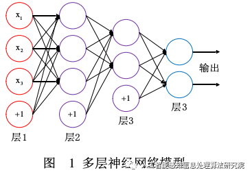
A neural network is formed by connecting numerous simple neurons together, where the output of one neuron can serve as the input of another. A multi-layer neural network model is often depicted as shown in Figure 1. For neural network models, the ultimate goal is to obtain the final optimized parameter model for classification, detection, and segmentation problems. Therefore, the most important part of a neural network model is the continuous optimization of its own model, and achieving this goal is primarily dependent on the forward and backward propagation algorithms.
(1) Forward Propagation Algorithm
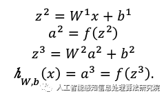
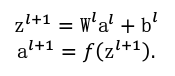
The above formula represents the forward propagation steps. Here, 𝑎(1)= 𝑥 is the activation value of the input layer, and the calculation method for the activation value 𝑎(𝑙+1) of the layer l + 1 is shown in the following formula:
(2) Backward Propagation Algorithm
The goal of the backward propagation algorithm is to minimize the function J(W,b) with W and b as parameters. To train the neural network, each parameter 𝑊i𝑗(𝑙) and each parameter 𝑏i(𝑙) will be initialized to random values, which are close to 0 and as small as possible, with the main purpose of breaking symmetry.
To perform forward propagation on (𝑥, 𝑦), it is necessary to first calculate the activation values of all nodes in the neural network, then compute the “residual” 𝛿(𝑙) for each node i in layer l, which represents the influence of this node on the overall output value. The final output node can directly obtain the activation value from the neural network and compare how far it is from the actual value, which can be defined as 𝛿(𝑛). Meanwhile, for the intermediate layer 𝑙, the residual 𝛿(𝑙) can be calculated from the weighted average of the residuals from layer 𝑙 + 1, using the nodes 𝑎(𝑙) as input. The specific steps are:
(a) Perform calculations using the forward propagation algorithm to obtain the activation values of 𝐿2, 𝐿3, … 𝐿𝑛𝑙.
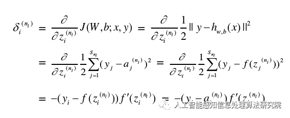
(b) The residual of each output node i in the nth layer can be calculated using the following formula:
(c) For 𝑙 = 𝑛− 1, 𝑛𝑙− 2, 𝑛𝑙− 3, … ,2, the residual of the i-th node in each layer can be calculated using the following formula:
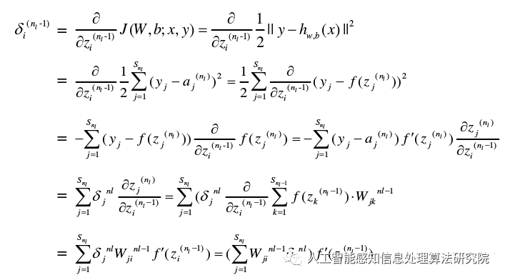
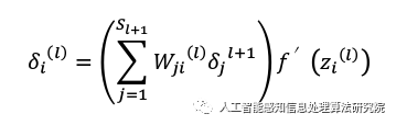
By changing the relationship of 𝑛− 1 and 𝑛𝑙 to the relationship of 𝑙 and 𝑙 + 1 in the above formulas, we can derive:
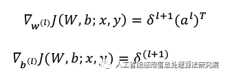
(d) Calculate the final required partial derivatives, as shown in the following formula:

These formulas can be expressed using matrix-vector notation:

2 Convolutional Neural Networks
Convolutional neural networks are feature extraction networks that typically consist of multiple convolutional layers and pooling layers, and usually end with fully connected layers. In convolutional neural networks, all weights are shared, and the pooling operation has translational invariance. Additionally, convolutional neural networks have fewer parameters compared to multi-layer neural networks and are much easier to train. The common architecture of convolutional neural networks is shown in the figure below.
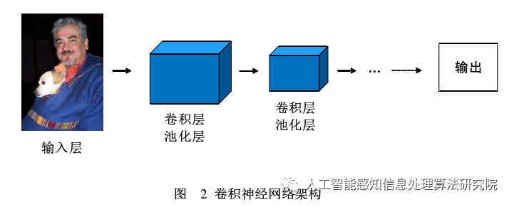
As shown in Figure 2, the architecture of convolutional neural networks typically includes an input layer, multiple convolutional layers, activation layers, and output sections. However, in general, we can design different convolutional neural network architectures according to different task requirements, hardware conditions, etc. The purpose of adding fully connected layers in the convolutional network structure is to perform classification predictions on given objects. In practice, we can use 1×1 convolutions to replace fully connected layers to reduce the number of parameters.
