Introduction
Using PyTorch to implement the ViT model code from scratch, training the ViT model on the CIFAR-10 dataset for image classification.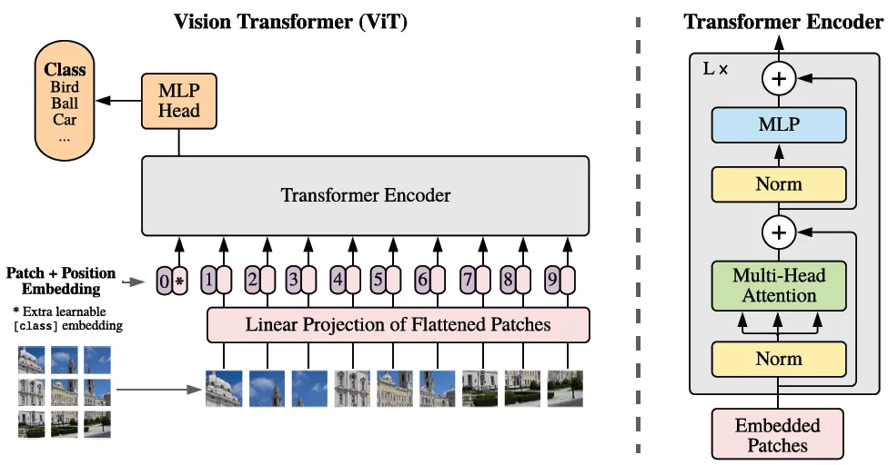
Architecture of ViT
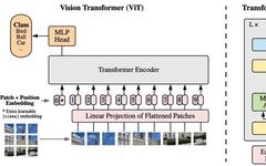
The architecture of ViT is inspired by BERT, which is an encoder-only transformer model typically used for supervised learning tasks in NLP such as text classification or named entity recognition. The main idea behind ViT is that images can be viewed as a series of patches, analogous to tokens in NLP tasks.

The input image is divided into small patches and then flattened into a sequence of vectors. These vectors are then processed by a transformer encoder, allowing the model to learn interactions between patches through a self-attention mechanism. The output from the transformer encoder is then fed into a classification layer that outputs the predicted class of the input image.
Code Implementation
Below is the PyTorch code implementation for various components of the model.
01
Image Embedding Transformation
To feed input images into the Transformer model, we need to convert the images into a series of vectors. This is done by segmenting the image into a non-overlapping grid of patches, and then linearly projecting these patches to obtain a fixed-size embedding vector for each patch. For this, we can use PyTorch’s layer: nn.Conv2d
class PatchEmbeddings(nn.Module):
    """
    Convert the image into patches and then project them into a vector space.
    """

    def __init__(self, config):
        super().__init__()
        self.image_size = config["image_size"]
        self.patch_size = config["patch_size"]
        self.num_channels = config["num_channels"]
        self.hidden_size = config["hidden_size"]
        # Calculate the number of patches from the image size and patch size
        self.num_patches = (self.image_size // self.patch_size) ** 2
        # Create a projection layer to convert the image into patches
        # The layer projects each patch into a vector of size hidden_size
        self.projection = nn.Conv2d(self.num_channels, self.hidden_size, kernel_size=self.patch_size, stride=self.patch_size)

    def forward(self, x):
        # (batch_size, num_channels, image_size, image_size) -> (batch_size, num_patches, hidden_size)
        x = self.projection(x)
        x = x.flatten(2).transpose(1, 2)
        return x
kernel_size=self.patch_size and ensure that the layer’s filters are applied to non-overlapping patches. stride=self.patch_sizeAfter the patches are converted to an embedding sequence, a [CLS] token is added to the beginning of the sequence, which will later be used for classification in the classification layer. The embedding of the [CLS] token is learned during training.Since patches from different positions may contribute differently to the final prediction, we also need a method to encode the positional information of the patches into the sequence. We will use learnable position embedding vectors to add positional information to the embedding vectors. This is similar to how positional embeddings are used in Transformer models for NLP tasks.
class Embeddings(nn.Module):
    def __init__(self, config):
        super().__init__()
        self.config = config
        self.patch_embeddings = PatchEmbeddings(config)
        # Create a learnable [CLS] token
        # Similar to BERT, the [CLS] token is added to the beginning of the input sequence
        # and is used to classify the entire sequence
        self.cls_token = nn.Parameter(torch.randn(1, 1, config["hidden_size"]))
        # Create position embeddings for the [CLS] token and the patch embeddings
        # Add 1 to the sequence length for the [CLS] token
        self.position_embeddings =
            nn.Parameter(torch.randn(1, self.patch_embeddings.num_patches + 1, config["hidden_size"]))
        self.dropout = nn.Dropout(config["hidden_dropout_prob"])

    def forward(self, x):
        x = self.patch_embeddings(x)
        batch_size, _, _ = x.size()
        # Expand the [CLS] token to the batch size
        # (1, 1, hidden_size) -> (batch_size, 1, hidden_size)
        cls_tokens = self.cls_token.expand(batch_size, -1, -1)
        # Concatenate the [CLS] token to the beginning of the input sequence
        # This results in a sequence length of (num_patches + 1)
        x = torch.cat((cls_tokens, x), dim=1)
        x = x + self.position_embeddings
        x = self.dropout(x)
        return x
In this step, the input image is transformed into an embedding sequence with positional information and is ready to be fed into the transformer layer.
02
Multi-Head Attention
Before introducing the transformer encoder, we first explore the multi-head attention module, which is a core component of it. Multi-head attention is used to compute interactions between different color blocks in the input image. Multi-head attention consists of multiple attention heads, each of which is an attention layer.Let’s implement the head of the multi-head attention module. This module takes a series of embedding vectors as input and computes the query, key, and value vectors for each embedding vector. Then, the attention weights for each token are calculated using the query and key vectors. Finally, the new embedding is computed as a weighted sum of the value vectors using the attention weights. We can think of this mechanism as a soft version of a database query, where the query vector looks up the most relevant key vectors in the database and retrieves the value vectors to compute the query output.
class AttentionHead(nn.Module):
    """
    A single attention head.
    This module is used in the MultiHeadAttention module.
    """
    def __init__(self, hidden_size, attention_head_size, dropout, bias=True):
        super().__init__()
        self.hidden_size = hidden_size
        self.attention_head_size = attention_head_size
        # Create the query, key, and value projection layers
        self.query = nn.Linear(hidden_size, attention_head_size, bias=bias)
        self.key = nn.Linear(hidden_size, attention_head_size, bias=bias)
        self.value = nn.Linear(hidden_size, attention_head_size, bias=bias)

        self.dropout = nn.Dropout(dropout)

    def forward(self, x):
        # Project the input into query, key, and value
        # The same input is used to generate the query, key, and value,
        # so it's usually called self-attention.
        # (batch_size, sequence_length, hidden_size) -> (batch_size, sequence_length, attention_head_size)
        query = self.query(x)
        key = self.key(x)
        value = self.value(x)
        # Calculate the attention scores
        # softmax(Q*K.T/sqrt(head_size))*V
        attention_scores = torch.matmul(query, key.transpose(-1, -2))
        attention_scores = attention_scores / math.sqrt(self.attention_head_size)
        attention_probs = nn.functional.softmax(attention_scores, dim=-1)
        attention_probs = self.dropout(attention_probs)
        # Calculate the attention output
        attention_output = torch.matmul(attention_probs, value)
        return (attention_output, attention_probs)
Then, the outputs of all attention heads are concatenated and linearly projected to obtain the final output of the multi-head attention module.
class MultiHeadAttention(nn.Module):    """    Multi-head attention module.    This module is used in the TransformerEncoder module.    """
    def __init__(self, config):        super().__init__()        self.hidden_size = config["hidden_size"]        self.num_attention_heads = config["num_attention_heads"]        # The attention head size is the hidden size divided by the number of attention heads        self.attention_head_size = self.hidden_size // self.num_attention_heads        self.all_head_size = self.num_attention_heads * self.attention_head_size        # Whether or not to use bias in the query, key, and value projection layers        self.qkv_bias = config["qkv_bias"]        # Create a list of attention heads        self.heads = nn.ModuleList([])        for _ in range(self.num_attention_heads):            head = AttentionHead(                self.hidden_size,                self.attention_head_size,                config["attention_probs_dropout_prob"],                self.qkv_bias            )            self.heads.append(head)        # Create a linear layer to project the attention output back to the hidden size        # In most cases, all_head_size and hidden_size are the same        self.output_projection = nn.Linear(self.all_head_size, self.hidden_size)        self.output_dropout = nn.Dropout(config["hidden_dropout_prob"])

    def forward(self, x, output_attentions=False):        # Calculate the attention output for each attention head        attention_outputs = [head(x) for head in self.heads]        # Concatenate the attention outputs from each attention head        attention_output = torch.cat([attention_output for attention_output, _ in attention_outputs], dim=-1)        # Project the concatenated attention output back to the hidden size        attention_output = self.output_projection(attention_output)        attention_output = self.output_dropout(attention_output)        # Return the attention output and the attention probabilities (optional)        if not output_attentions:            return (attention_output, None)        else:            attention_probs = torch.stack([attention_probs for _, attention_probs in attention_outputs], dim=1)            return (attention_output, attention_probs)
03
Encoder
The encoder consists of a stack of MHA + MLP. Each transformer layer mainly consists of the multi-head attention module we just implemented and a feed-forward network. To better scale the model and stabilize training, two Layer normalization layers and skip connections are added to the transformer layer.Let’s implement a transformer layer (referred to as Block in the code, as it is a building block of the transformer encoder). We will start with the feed-forward network, which is a simple two-layer MLP with a GELU activation in between.
class MLP(nn.Module):    """    A multi-layer perceptron module.    """    def __init__(self, config):        super().__init__()        self.dense_1 = nn.Linear(config["hidden_size"], config["intermediate_size"])        self.activation = NewGELUActivation()        self.dense_2 = nn.Linear(config["intermediate_size"], config["hidden_size"])        self.dropout = nn.Dropout(config["hidden_dropout_prob"])
    def forward(self, x):        x = self.dense_1(x)        x = self.activation(x)        x = self.dense_2(x)        x = self.dropout(x)        return x
We have implemented multi-head attention and MLP, and we can combine them to create a transformer layer. Skip connections and layer normalization will be applied to the input of each layer.
class Block(nn.Module):    """    A single transformer block.    """    def __init__(self, config):        super().__init__()        self.attention = MultiHeadAttention(config)        self.layernorm_1 = nn.LayerNorm(config["hidden_size"])        self.mlp = MLP(config)        self.layernorm_2 = nn.LayerNorm(config["hidden_size"])
    def forward(self, x, output_attentions=False):        # Self-attention        attention_output, attention_probs =
            self.attention(self.layernorm_1(x), output_attentions=output_attentions)        # Skip connection        x = x + attention_output        # Feed-forward network        mlp_output = self.mlp(self.layernorm_2(x))        # Skip connection        x = x + mlp_output        # Return the transformer block's output and the attention probabilities (optional)        if not output_attentions:            return (x, None)        else:            return (x, attention_probs)
The transformer encoder stacks multiple transformer layers sequentially:
class Encoder(nn.Module):    """    The transformer encoder module.    """    def __init__(self, config):        super().__init__()        # Create a list of transformer blocks        self.blocks = nn.ModuleList([])        for _ in range(config["num_hidden_layers"]):            block = Block(config)            self.blocks.append(block)
    def forward(self, x, output_attentions=False):        # Calculate the transformer block's output for each block        all_attentions = []        for block in self.blocks:            x, attention_probs = block(x, output_attentions=output_attentions)            if output_attentions:                all_attentions.append(attention_probs)        # Return the encoder's output and the attention probabilities (optional)        if not output_attentions:            return (x, None)        else:            return (x, all_attentions)
04
Building the ViT Model
After inputting the image into the embedding layer and transformer encoder, we obtain new embeddings for the image patches and the [CLS] token. At this point, the embeddings should contain some useful signals for classification after being processed by the transformer encoder. Similar to BERT, we will only pass the embedding of the [CLS] token to the classification layer.The classification layer is a fully connected layer that takes the [CLS] embedding as input and outputs the logits for each image. The following code implements the ViT model for image classification:
class ViTForClassfication(nn.Module):    """    The ViT model for classification.    """    def __init__(self, config):        super().__init__()        self.config = config        self.image_size = config["image_size"]        self.hidden_size = config["hidden_size"]        self.num_classes = config["num_classes"]        # Create the embedding module        self.embedding = Embeddings(config)        # Create the transformer encoder module        self.encoder = Encoder(config)        # Create a linear layer to project the encoder's output to the number of classes        self.classifier = nn.Linear(self.hidden_size, self.num_classes)        # Initialize the weights        self.apply(self._init_weights)
    def forward(self, x, output_attentions=False):        # Calculate the embedding output        embedding_output = self.embedding(x)        # Calculate the encoder's output        encoder_output, all_attentions = self.encoder(embedding_output, output_attentions=output_attentions)        # Calculate the logits, take the [CLS] token's output as features for classification        logits = self.classifier(encoder_output[:, 0])        # Return the logits and the attention probabilities (optional)        if not output_attentions:            return (logits, None)        else:            return (logits, all_attentions)
References
The code is actually compiled and translated from GitHub (I think it is very easy to understand, and anyone with a basic knowledge of PyTorch can comprehend it), if interested, you can check it out here:
https://github.com/lukemelas/PyTorch-Pretrained-ViT/blob/master/pytorch_pretrained_vit/transformer.py
https://tintn.github.io/Implementing-Vision-Transformer-from-Scratch/