Deep Learning Text Representation Models

Source: Poll’s Notes

Original URL:http://www.cnblogs.com/maybe2030/

Reading Directory

1. Word Vectors
2. Distributed Representation of Word Vectors
3. Word Vector Models
4. Word2Vec Algorithm Concepts
5. Doc2Vec Algorithm Concepts
6. References

Deep learning has opened a new chapter in machine learning, and significant breakthroughs have been made in applying deep learning to images and speech. Deep learning is often praised as an artificial intelligence algorithm similar to the structure of the human brain. However, why has deep learning not made substantial progress in the field of semantic analysis?

To quote a netizen from three years ago:

“Steve Renals calculated the number of accepted ICASSP papers that included ‘deep learning’ in their titles and found 44 papers, while NAACL had 0. There is a saying that language (words, sentences, texts, etc.) belongs to high-level cognitive abstract entities generated during human cognition, while speech and images belong to lower-level raw input signals, so the latter two are more suitable for deep learning to learn features.”

In fact, as of now, research in Deep Learning in the NLP field has already torn away a layer of mystery from the profound human language. The most interesting and fundamental aspect is the “word vector.”

1. Word Vectors

To convert the problem of natural language understanding into a machine learning problem, the first step is to find a way to mathematically represent these symbols. The most intuitive and, so far, the most commonly used word representation method in NLP is One-hot Representation, which represents each word as a long vector. This vector’s dimension is the size of the vocabulary, with the vast majority of elements being 0, and only one dimension having a value of 1, representing the current word. For example, “microphone” is represented as [0 0 0 1 0 0 0 0 0 0 0 0 0 0 0 0 …] and “Mike” is represented as [0 0 0 0 0 0 0 0 1 0 0 0 0 0 0 0 …]. Each word is a 1 in a sea of 0s. This One-hot Representation can be stored in a sparse way, which is very concise: assigning a numeric ID to each word. For instance, in the previous example, “microphone” is assigned 3 and “Mike” is assigned 8 (assuming counting starts from 0). If implemented in programming, a hash table can be used to assign a number to each word. This concise representation, combined with algorithms such as Maximum Entropy, SVM, CRF, etc., has effectively accomplished various mainstream tasks in the NLP field. However, this representation method also has a significant problem known as the “vocabulary gap” phenomenon: any two words are isolated from each other. Looking at these two vectors, it is impossible to see whether the two words are related, even synonyms like “microphone” and “Mike” cannot escape this issue. Additionally, this representation method can easily suffer from the curse of dimensionality, especially in some applications related to Deep Learning.

2. Distributed Representation of Word Vectors

Since the aforementioned intuitive One-hot Representation of word vectors has such significant drawbacks, a representation method that can represent the words themselves while considering semantic distance is needed, which is the Distributed Representation of word vectors that we will introduce next.

Distributed representation was first proposed by Hinton in 1986. It is a low-dimensional real-valued vector, generally looking like this:

[0.792, −0.177, −0.107, 0.109, −0.542, …]

Dimensions of 50 and 100 are quite common; of course, this vector representation is not unique. The greatest contribution of Distributed Representation is that related or similar words are brought closer together in distance. The distance between vectors can be measured using the most traditional Euclidean distance or cosine angle. Using this representation, the distance between “Mike” and “microphone” is much smaller than that between “Mike” and “weather.” Ideally, the representations of “Mike” and “microphone” should be exactly the same, but due to some people writing the English name “Mike” as “Mike,” the word “Mike” carries some semantic associations with a person’s name, thus not being completely identical to “microphone.”

Mapping words into a new space and representing them as multidimensional continuous real-valued vectors is called “Word Representation” or “Word Embedding.” Since the 21st century, people have gradually transitioned from the original sparse representation of word vectors to the current dense representation in low-dimensional space. Sparse representation often encounters the curse of dimensionality when solving practical problems and fails to express semantic information, failing to reveal the potential relationships between words. Low-dimensional space representation not only solves the curse of dimensionality but also uncovers the associative attributes between words, thus improving the semantic accuracy of the vectors.

3. Word Vector Models

a) LSA Matrix Decomposition Model

It employs the singular value decomposition method from linear algebra, selecting a few of the larger singular values corresponding feature vectors to map the original matrix to low-dimensional space, thus achieving word vectorization.

b) PLSA Latent Semantic Analysis Probability Model

This model re-examines the matrix decomposition model from the perspective of probability and derives a word vector model equivalent to LSA from a statistical and probabilistic perspective.

c) LDA Document Generation Model

According to the document generation process, using Bayesian estimation statistical methods, documents are represented by multiple topics. LDA not only solves the synonym problem but also addresses the issue of polysemy. The training methods for LDA models include the original paper’s EM-based and differential Bayesian methods, as well as the later Gibbs Sampling algorithms.

d) Word2Vector Model

This algorithm, which has just gained popularity in recent years, trains an N-gram language model through neural network machine learning algorithms and derives the corresponding vectors for words during the training process. This article will detail the principles of this method.

4. Word2Vec Algorithm Concepts

What is Word2Vec? You can understand it as an efficient algorithm model that represents words as real-valued vectors, which uses the ideas of deep learning to simplify the processing of text content into vector operations in K-dimensional vector space, where the similarity in the vector space can be used to represent the semantic similarity of the text.

The word vectors output by Word2Vec can be used for many NLP-related tasks, such as clustering, finding synonyms, part-of-speech analysis, etc. Alternatively, treating words as features, Word2Vec can map features into K-dimensional vector space, seeking deeper feature representations for text data.

The word vectors used by Word2Vec are not the One-hot Representation type mentioned above but are of the Distributed Representation type. The basic idea is to train to map each word into a K-dimensional real-valued vector (K is generally a hyperparameter in the model) and use the distance between words (such as cosine similarity, Euclidean distance, etc.) to determine their semantic similarity. It employs a three-layer neural network: input layer – hidden layer – output layer. A core technology is to use Huffman coding based on word frequency, so that the content activated in the hidden layer of words with similar frequencies is basically consistent; words that appear more frequently have fewer hidden layer activations, effectively reducing computational complexity. One reason for Word2Vec’s popularity is its efficiency; Mikolov pointed out in the paper that an optimized single-machine version can train thousands of billions of words in a day.

This three-layer neural network itself models the language model while also obtaining a representation of words in vector space; this side effect is the true goal of Word2Vec.

Compared to the classic processes of Latent Semantic Analysis (LSI) and Latent Dirichlet Allocation (LDA), Word2Vec utilizes the context of words, making the semantic information richer.

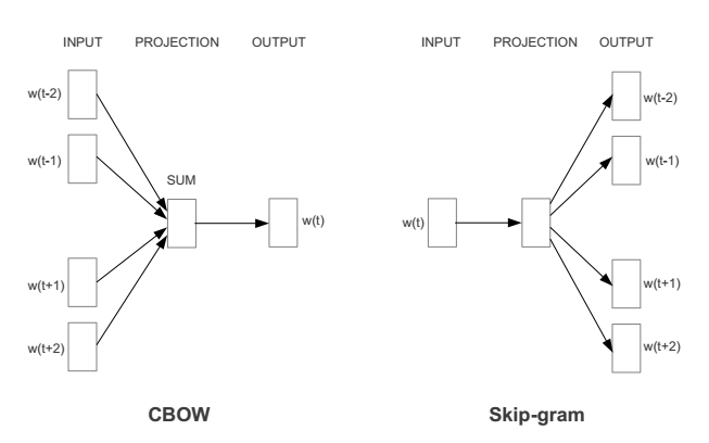
Word2Vec actually consists of two different methods: Continuous Bag of Words (CBOW) and Skip-gram. The goal of CBOW is to predict the probability of the current word based on context. Skip-gram, on the other hand, predicts the context’s probability based on the current word (as shown in the figure below). Both methods use artificial neural networks as their classification algorithms. Initially, each word is a random N-dimensional vector. After training, the algorithm uses either CBOW or Skip-gram to obtain the optimal vector for each word.

Taking a suitably sized window as context, the input layer reads the words within the window, summing their vectors (K-dimensional, initially random) to form K nodes in the hidden layer. The output layer is a large binary tree, with leaf nodes representing all words in the corpus (if the corpus contains V independent words, the binary tree has |V| leaf nodes). The algorithm for constructing this entire binary tree is the Huffman tree. Thus, for each leaf node representing a word in the corpus, there will be a globally unique code, such as “010011”; let’s say the left subtree is 1 and the right subtree is 0. Next, each node in the hidden layer will connect to the internal nodes of the binary tree, so each internal node of the binary tree will have K edges, each with a weight.

For a word w_t in the corpus, corresponding to a leaf node in the binary tree, it must have a binary code, such as “010011”. During the training phase, when given context, to predict the subsequent word w_t, we start traversing from the root node of the binary tree. The goal here is to predict each bit of the binary number of this word. In other words, for the given context, our goal is to maximize the probability of predicting the binary code of the word. Figuratively, we hope that at the root node, the probability of the word vector connecting to the root node and resulting in bit=1 is as close to 0 as possible; at the second layer, we hope its bit=1 probability is as close to 1 as possible, and so on. The probabilities calculated along the way are multiplied together, yielding the probability P(w_t) of the target word under the current network. For the current sample, the residual is 1-P(w_t), allowing us to use gradient descent to train this network to obtain all parameter values. It is evident that the final probability value calculated according to the binary code of the target word is normalized.

Hierarchical Softmax constructs a binary tree using Huffman coding, effectively employing the idea of approximating multi-class classification with a series of binary classifications. For example, if we treat all words as outputs, then “orange” and “car” are mixed together. Given the context of w_t, the model first determines whether w_t is a noun, then whether it is food, then whether it is fruit, and finally whether it is “orange”.

During the training process, the model assigns appropriate vectors to these abstract intermediate nodes, representing all child nodes. Since the actual words share the vectors of these abstract nodes, the Hierarchical Softmax method and the original problem are not equivalent, but this approximation does not significantly degrade performance while significantly increasing the scale of the model’s solution.

If this binary tree is not used, and instead, the probability of each output is calculated directly from the hidden layer—i.e., traditional Softmax—then it needs to compute for each word in |V|, which has a time complexity of O(|V|). Using a binary tree (such as the Huffman tree in Word2Vec) reduces the time complexity to O(log2(|V|)), greatly speeding up the process.

Now these word vectors have captured contextual information. We can use basic algebraic formulas to discover relationships between words (for example, “king” – “man” + “woman” = “queen”). These word vectors can replace bag-of-words models to predict the sentiment of unknown data. The advantage of this model is that it not only considers contextual information but also compresses the data size (typically, the vocabulary size is around 300 words instead of the previous model’s 100,000 words). Since neural networks can extract these feature information for us, we only need to do minimal manual work. However, due to the varying lengths of texts, we may need to use the average of all word vectors as input values for classification algorithms to classify the entire text document.

5. Doc2Vec Algorithm Concepts

However, even if the above model averages the word vectors, we still overlook the impact of the order of words on sentiment analysis. The above Word2Vec is based on word dimensions for “semantic analysis” and does not possess the capability for contextual “semantic analysis”.

As a summarizing method for processing variable-length texts, Quoc Le and Tomas Mikolov proposed the Doc2Vec method. Apart from adding a paragraph vector, this method is almost identical to Word2Vec. Like Word2Vec, this model also has two methods: Distributed Memory (DM) and Distributed Bag of Words (DBOW). DM tries to predict the probability of words given the context and paragraph vector. During the training process of a sentence or document, the paragraph ID remains unchanged, sharing the same paragraph vector. DBOW predicts the probability of a set of random words in the paragraph given only the paragraph vector.

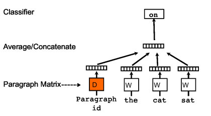
First, let’s look at the CBOW method. Compared to the CBOW model of Word2Vec, the differences are:

During training, a paragraph ID is added, meaning each sentence in the training corpus has a unique ID. The paragraph ID, like ordinary words, is also mapped to a vector, namely the paragraph vector. The dimensions of the paragraph vector and the word vector are the same, but they come from two different vector spaces. In subsequent calculations, the paragraph vector and word vector are summed or concatenated to be used as input to the output layer’s softmax. During the training process of a sentence or document, the paragraph ID remains unchanged, sharing the same paragraph vector, effectively utilizing the entire sentence’s semantics when predicting the probability of words.
In the prediction phase, a new paragraph ID is assigned to the sentence to be predicted, and the parameters of the word vector and output layer’s softmax remain unchanged from those obtained during training, reusing gradient descent to train the sentence to be predicted. Once convergence is achieved, the paragraph vector for the sentence to be predicted is obtained.

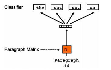
Sentence2vec, compared to the skip-gram model of Word2Vec, has the difference that in sentence2vec, the input is the paragraph vector, and the output is the randomly sampled words from that paragraph.

Below is an example of the results of sentence2vec. First, train the sentence vectors using Chinese sentence corpus, and then calculate the cosine values between sentence vectors to obtain the most similar sentences. It can be seen that the sentence vectors are quite impressive in representing the semantics of sentences.

6. References

1. Official Word2Vec Address: Word2Vec Homepage

2. Python version of Word2Vec implementation: gensim word2vec

3. Python version of Doc2Vec implementation: gensim doc2vec

4. A New Method for Sentiment Analysis—Based on Word2Vec/Doc2Vec/Python

5. Turning Numbers into Gold: Some Methods of Semantic Analysis (Middle Part)

6. Wang Lin’s Introduction to the Principles of Word2Vec

Thank you for sharing and supporting!