Click on the above“Beginner Learning Vision”, select to add “Star Mark” or “Top”
Heavyweight content delivered at the first time
Author: helton_yan@CSDN (Authorized)Source: https://blog.csdn.net/SESESssss/article/details/114340066
Abstract
This article reproduces the classic Backbone structures Inception v1, ResNet-50, and FPN, and shares some network building tips based on PyTorch, very detailed and informative! >> Join the Extreme City CV Technology Exchange Group, stay at the forefront of computer vision
Article Directory
-
1.VGG
-
1.1 Improvements:
-
1.2 PyTorch Reproduction of VGG19
-
1.2.1 Tips:
-
1.2.2 Print Network Information:
-
Inception (GoogLeNet)
-
2.1 Improvements (Inception v1)
-
2.2.2 Improvements (Inception v2)
-
2.2 PyTorch Reproduction of Inception v1:
-
2.2.1 Overall Framework of the Network:
-
2.2.2 Parameters of Each Layer:
-
2.2.3 PyTorch Reproduction of Inception Basic Module
-
2.2.4 Tips
-
ResNet
-
3.1 Improvements
-
3.2 PyTorch Reproduction of ResNet-50
-
3.2.1 Overall Architecture of ResNet-50
-
3.2.2 Bottleneck Structure
-
3.2.3 ResNet-50 Diagram and Layer Parameter Details
-
3.2.4 Implementing a Bottleneck Module:
-
3.2.5 Implementing ResNet-50
-
FPN (Feature Pyramid)
-
4.1 Semantic Information of Features
-
4.2 Improvements
-
4.3 PyTorch Reproduction of FPN
-
4.3.1 FPN Network Architecture
-
4.3.2 Reproducing the FPN Network
Introduction
The development of convolutional neural networks began in the last century. Let’s take a trip back to 1998, when Professor Yann LeCun proposed a relatively mature convolutional neural network architecture LeNet-5, which is now regarded as the “Hello World” of convolutional neural networks. However, due to the limitations of computing power at that time and the rise of support vector machines (kernel learning methods), CNN methods were not recognized as mainstream methods in the academic community. Fast forward 14 years to 2012, when AlexNet won the ImageNet image recognition competition with an accuracy rate about 10% higher than the second place, completely igniting the research boom in deep learning and convolutional neural networks. From then on, CNN entered a phase of rapid development, becoming the mainstream framework in computer vision, and various CNN-based image recognition networks began to shine.
This blog will introduce some classic CNN networks that are very well-known in the field of image recognition today. Although convolutional network frameworks have become increasingly complex with in-depth research, we can still find their traces in some of the latest network structures. These classic CNN networks are sometimes the backbone of the entire algorithm for feature extraction (the quality of features often directly affects the accuracy of classification; features with stronger expressive power can also bring stronger classification ability to the model), hence they are also referred to as Backbone.
This blog reproduces classic Backbone structures based on code practice and shares some network building tips based on PyTorch.
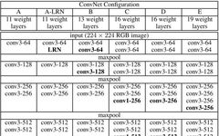
1.VGG
Network Architecture:
The VGG16 network consists of 13 convolutional layers + 3 fully connected layers.
1.1 Improvements:
-
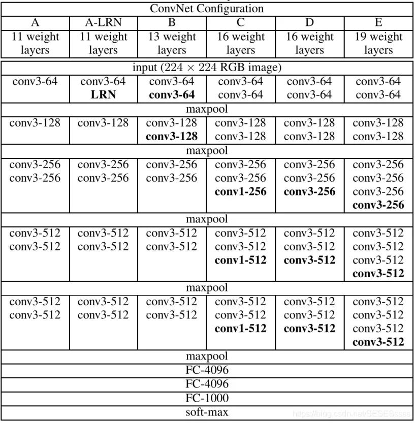
Smaller Convolution Kernels, compared to AlexNet, the convolution kernel size used in VGG network does not exceed 3×3. This structure has an advantage over larger convolution kernels: stacking two 3×3 convolution kernels has a receptive field (the amount of information fused into one pixel of the feature map determines the size of the receptive field) equivalent to a 5×5 convolution kernel (as shown in the figure), and under the same receptive field conditions, adding activation functions between two 3×3 convolutions enhances the non-linear capability compared to a single 5×5 convolution.
-
Deeper Network Structure, compared to AlexNet with only 5 convolutional layers, the VGG series deepens the network’s depth, which helps the network extract more complex semantic information from images.
1.2 PyTorch Reproduction of VGG19
class VGG19(nn.Module):
    def __init__(self, num_classes = 1000):  # num_classes number of pre-defined categories

        super(VGG19, self).__init__()

        # Construct feature extraction layers:
        feature_layers = []  # Store convolution layers in a list
        in_dim = 3  # Input is a three-channel image
        out_dim = 64  # Output feature depth is 64

        # Use a loop to construct, avoiding redundancy in code for deep networks:
        for i in range(16):  # VGG19 has a total of 16 convolution layers
            feature_layers += [nn.Conv2d(in_dim, out_dim, 3, 1, 1), nn.ReLU(inplace = True)]  # Basic structure: convolution + activation function
            in_dim = out_dim
            # Add max pooling after the 2nd, 4th, 8th, 12th, 16th convolution layers:
            if i == 1 or i == 3 or i == 7 or i == 11 or i == 15:
                feature_layers += [nn.MaxPool2d(2)]
                if i < 11:
                    out_dim *= 2
        self.features = nn.Sequential(*feature_layers)
        # * indicates a variable number of parameters, otherwise it will report an error that the list is not a Module subclass


        # Fully connected layer classification:
        self.classifier = nn.Sequential(
            nn.Linear(512 * 7 * 7, 4096),
            nn.ReLU(inplace = True),
            nn.Dropout(),
            nn.Linear(4096, 4096),
            nn.ReLU(inplace = True),
            nn.Dropout(),
            nn.Linear(4096, num_classes),
        )

    # Forward propagation
    def forward(self, x):
        x = self.features(x)
        x = x.view(x.size(0), -1)
        x = self.classifier(x)
        return x
1.2.1 Tips:
-
When the structure of the network is repetitive, use a for loop to avoid redundancy in code form
-
Encapsulate networks with different functions into a large Sequential module for clarity
-
Convolution operation output size calculation formula: Out=(In-Kernel+2Padding)/Stride+1 (Kernel: convolution kernel size, Stride: step size, Padding: boundary padding) To ensure the output size is consistent with the original size, Padding can be set to:Padding = (kernel-1)/2)
-
The output size calculation formula for pooling operations is the same as for convolution operations
-
In the actual implementation of convolution and fully connected computations in deep learning frameworks, they are essentially matrix operations:
If the depth of the input feature map is N and the output feature map depth is M, then the dimension of the convolution kernel is:NxMxKxK (K being the size of the convolution kernel). Therefore, fully convolutional networks have no requirements on the size of the input image.
The size of the fully connected layer is related to the size of the input features (flattening the feature map into a one-dimensional vector). If the input feature vector is 1xN, the output is 1xM, then the dimension of the fully connected layer is:MxN.
1.2.2 Print Network Information:
Use torch.summary to output the network architecture:
vgg19 = VGG19()

#print(vgg19) # Output the network architecture
summary(vgg19, input_size = [(3, 224, 224)]) # Output the network architecture, feature size of each layer, and network parameters
Output the size of each layer of the network:
for param in vgg19.parameters(): # Output the size of each layer of the network
    print(param.size())


batch_size = 16
input = torch.randn(batch_size, 3, 224, 224) # Build a random data to simulate a batch size
output = vgg19(input)
print(output.shape)  # torch.Size([16, 1000])
2.Inception (GoogLeNet)
2.1 Improvements (Inception v1)
Shortcomings of previous networks:
- Increased network parameters due to deeper depth
- Deeper networks require more training data and are prone to overfitting
- Deeper networks are prone to gradient vanishing during training
Improvements:
-
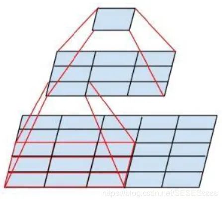
Introduced the Inception module as the basic module of the network, stacking the overall network based on the basic module; used channel concatenation (Concat) to merge features extracted by different convolution kernels
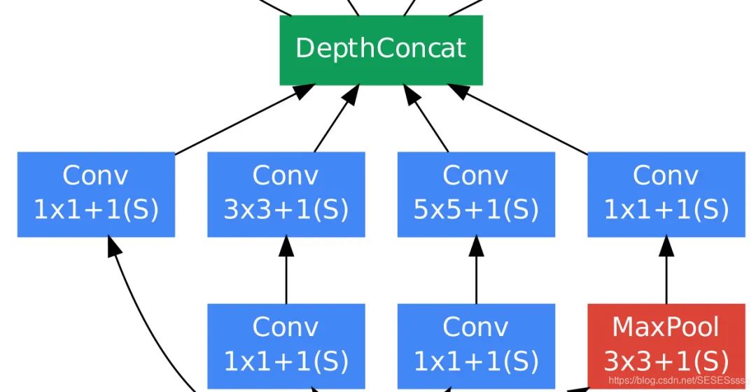
The basic Inception module is shown in the figure, using three different sizes of convolution kernels for convolution operations, and also includes a max pooling layer. Finally, the results output from these four parts are concatenated and passed to the next layer:
-
Used 1×1 convolution for dimensionality reduction (reducing depth) to decrease the number of training parameters.
This structure has a drawback, that is, the input channel number of one branch in the module is the sum of the output channel numbers of all branches from the previous module (channel merging). After stacking multiple modules, the calculated parameter amount becomes massive. To solve this problem, the author added a 1×1 convolution layer before the convolution layer of each branch to reduce the channel count.
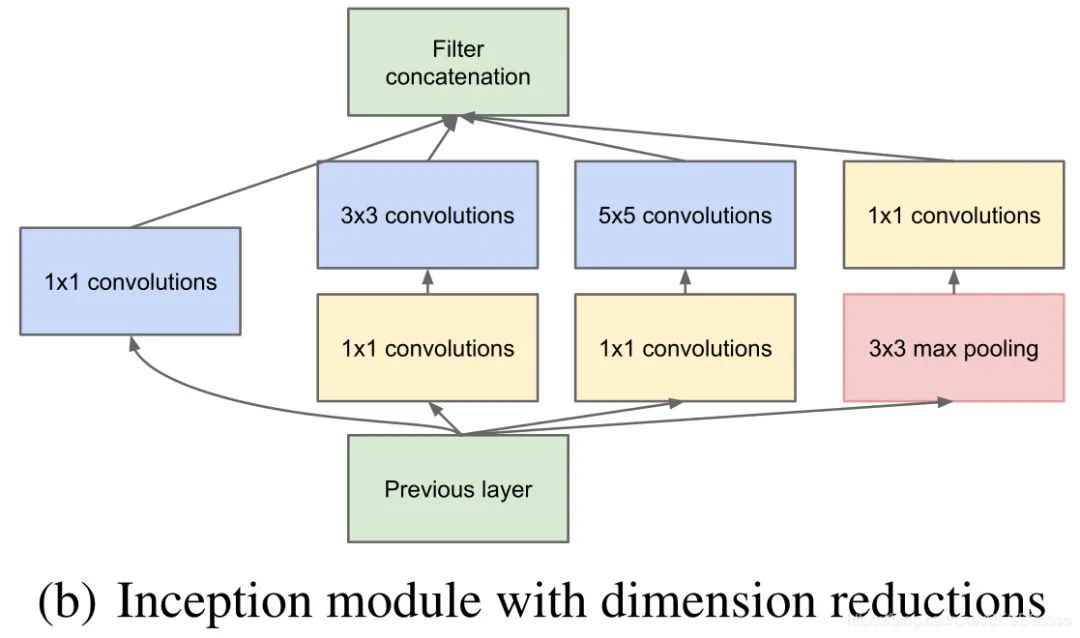
You might wonder why not directly reduce the feature dimension on the outputs of 3×3 or 5×5 convolutions instead of using 1×1 convolutions. (The author believes that this approach can enhance the network’s non-linear capability because there are activation functions between convolutions)
-
Introduced auxiliary classifiers (calculate classification loss at different depths and backpropagate together)
The author found that the features of the intermediate layers differ greatly from those of the deeper layers. Therefore, during training, two auxiliary classifiers were added to the intermediate layers. The results of the auxiliary classifiers are calculated along with the output results, and the loss of the auxiliary classifiers accounts for 0.3 of the total loss of the network. The author believes that this structure helps enhance the classification ability of the network on shallower features, **equivalent to adding an additional constraint (regularization) to the network**, and during inference, the structures of these auxiliary networks will be discarded.
2.2.2 Improvements (Inception v2)
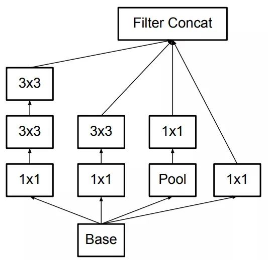
Convolution Decomposition
Inception v2 decomposes the large 5×5 convolution into two smaller 3×3 convolutions (imitating the processing method of VGG network, reducing the parameter amount while increasing the non-linear capability of the network), and adds BN layers:
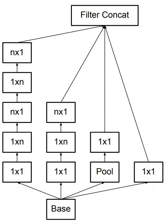
Furthermore, Inception v2 decomposes nxn convolutions into two 1xn and nx1 convolutions (spatially separable convolution), further reducing network parameters while maintaining the same receptive field:
References:
Inception series Inception_v2-v3: https://www.cnblogs.com/wxkang/p/13955363.html
[Paper Notes] Xception: https://zhuanlan.zhihu.com/p/127042277
2.2 PyTorch Reproduction of Inception v1:
2.2.1 Overall Framework of the Network:
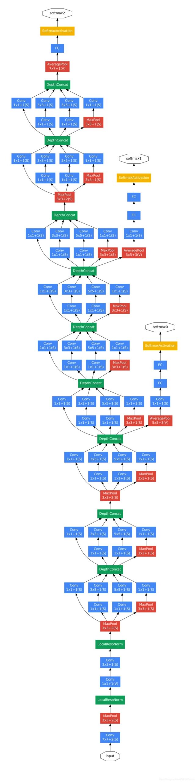
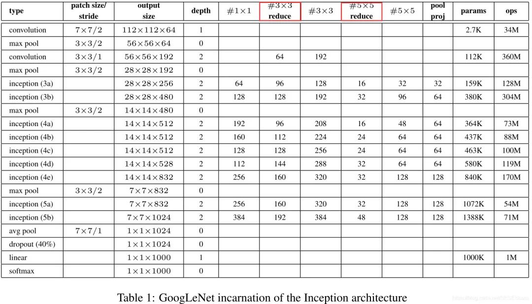
2.2.2 Parameters of Each Layer:
The red box indicates the 1×1 convolution used for feature dimensionality reduction.
2.2.3 PyTorch Reproduction of Inception Basic Module
Encapsulate convolution + activation function as a basic convolution group:
# Encapsulate Conv + ReLU into a basic class:
class BasicConv2d(nn.Module):
    def __init__(self, in_channel, out_channel, kernel_size, stride=1, padding=0):
        super(BasicConv2d, self).__init__()
        self.conv = nn.Sequential(
            nn.Conv2d(in_channel, out_channel, kernel_size,
                      stride=stride, padding=padding),
            nn.ReLU(True)
        )

    def forward(self, x):
        x = self.conv(x)
        return x
Construct an Inception module:
# Construct Inception basic module:
class Inception(nn.Module):
    def __init__(self, in_dim, out_1x1, out_3x3_reduce, out_3x3, out_5x5_reduce, out_5x5, out_pool):
        super(Inception, self).__init__()
        # Branch 1:
        self.branch_1x1 = BasicConv2d(in_dim, out_1x1, 1)
        # Branch 2:
        self.branch_3x3 = nn.Sequential(
            BasicConv2d(in_dim, out_3x3_reduce, 1),
            BasicConv2d(out_3x3_reduce, out_3x3, 3, padding=1),
        )
        # Branch 3:
        self.branch_5x5 = nn.Sequential(
            BasicConv2d(in_dim, out_5x5_reduce, 1),
            BasicConv2d(out_5x5_reduce, out_5x5, 5, padding=2),
        )
        # Branch 4:
        self.branch_pool = nn.Sequential(
            nn.MaxPool2d(3, stride=1, padding=1),
            BasicConv2d(in_dim, out_pool, 1),
        )

    def forward(self, x):
        b1 = self.branch_1x1(x)
        b2 = self.branch_3x3(x)
        b3 = self.branch_5x5(x)
        b4 = self.branch_pool(x)

        output = torch.cat((b1, b2, b3, b4), dim=1)  # Four modules concatenated along the feature map channel direction
        return output
Build the complete Inception v1:
# Build Inception v1:
class Inception_v1(nn.Module):
    def __init__(self, num_classes=1000, state="test"):
        super(Inception_v1, self).__init__()
        self.state = state
        self.block1 = nn.Sequential(
            BasicConv2d(3, 64, 7, stride=2, padding=3),
            nn.MaxPool2d(kernel_size=3, stride=2, padding=1),
            nn.LocalResponseNorm(64),
            BasicConv2d(64, 64, 1),
            BasicConv2d(64, 192, 3, padding=1),
            nn.LocalResponseNorm(192),
            nn.MaxPool2d(kernel_size=3, stride=2, padding=1),
        )
        self.block2 = nn.Sequential(
            Inception(192, 64, 96, 128, 16, 32, 32),
            Inception(256, 128, 128, 192, 32, 96, 64),
            nn.MaxPool2d(kernel_size=3, stride=2, padding=1),
            Inception(480, 192, 96, 208, 16, 48, 64),
        )
        self.block3 = nn.Sequential(
            Inception(512, 160, 112, 224, 24, 64, 64),
            Inception(512, 128, 128, 256, 24, 64, 64),
            Inception(512, 112, 144, 288, 32, 64, 64),
        )
        self.block4 = nn.Sequential(
            nn.MaxPool2d(kernel_size=3, stride=2, padding=1),
            Inception(528, 256, 160, 320, 32, 128, 128),
            Inception(832, 256, 160, 320, 32, 128, 128),
            Inception(832, 384, 192, 384, 48, 128, 128),
            nn.AvgPool2d(3, stride=1),
        )
        self.classifier = nn.Linear(4096, num_classes)

        if state == "train":
            # Two auxiliary classifiers:
            self.aux_classifier1 = Inception_classify(
                192 + 208 + 48 + 64, num_classes)
            self.aux_classifier2 = Inception_classify(
                112 + 288 + 64 + 64, num_classes)

    def forward(self, x):
        x = self.block1(x)
        x = self.block2(x)
        # Insert auxiliary classifier layer 1
        if self.state == 'train':
            aux1 = self.aux_classifier1(x)
        x = self.block3(x)
        # Insert auxiliary classifier layer 2
        if self.state == 'train':
            aux2 = self.aux_classifier2(x)
        x = self.block4(x)
        x = x.view(x.size(0), -1)
        out = self.classifier(x)

        if self.state == 'train':
            return aux1, aux2, out
        else:
            return out
2.2.4 Tips
When building a relatively complex network, encapsulate some basic modules that are reused into a basic class (for clarity).
3.ResNet
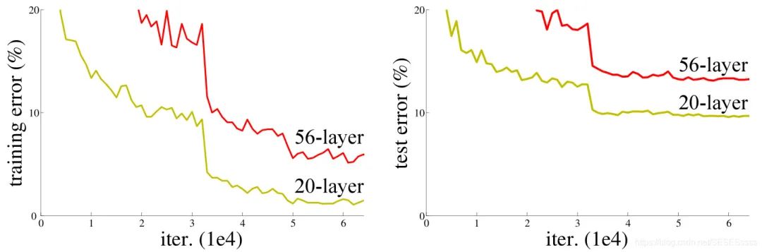
Based on past experience, it is generally believed that increasing the number of layers in a network can enhance its learning ability. Even if networks are prone to overfitting or gradient vanishing problems, existing methods can address these issues by increasing the dataset, using Dropout or regularization, or adding BN layers. However, experimental data has shown that even with effective measures to suppress overfitting or gradient vanishing, the accuracy of the network tends to decrease as the depth increases, and this is not due to overfitting (experimental data indicates that the training loss of deeper networks is actually higher).
In fact, one major factor hindering the depth of networks is the inability of gradients to propagate effectively, as the deeper the network, the poorer the gradient correlation during backpropagation, approaching white noise, leading to gradient updates that are essentially random disturbances.
What problem is ResNet solving? https://www.zhihu.com/question/64494691
To illustrate, it’s like the game of telephone we played as children; as the number of participants increases, the information spoken by the last person often diverges significantly from the original message.
3.1 Improvements
The previous bottleneck was the uncontrollable gradient vanishing in deep networks, the gradient correlation between deep and shallow networks decreased, making the network difficult to train.
ResNet’s improvement: introduces a residual mapping structure to solve the network degradation problem:
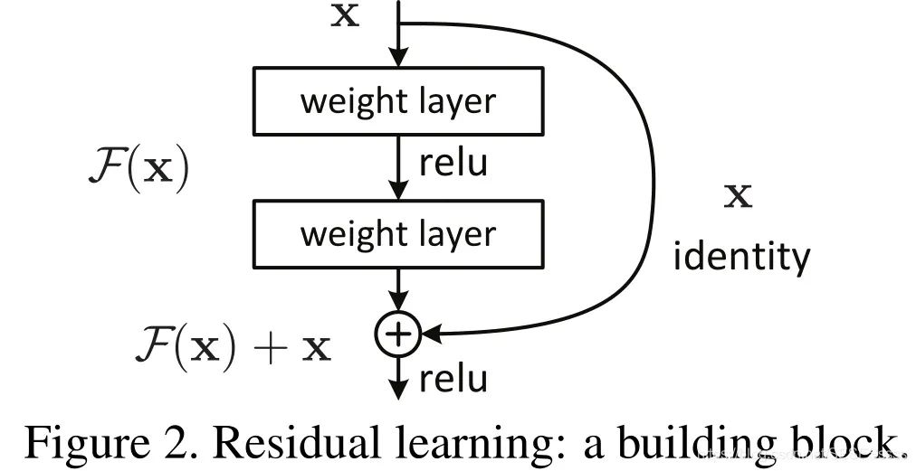
What is a residual mapping?
Assuming the input feature is x, the expected output feature is H(x). We know that for a typical neural network, each layer’s purpose is to perform a non-linear transformation on the input x, mapping the feature x as close to H(x) as possible, meaning the network needs to directly fit the output H(x).
However, with residual mapping, the module introduces a shortcut branch (identity mapping), transforming the mapping that the network needs to fit into a residual F(x): F(x) = H(x) – x.
The author hypothesizes in the paper that optimizing the residual mapping F(x) can effectively alleviate the gradient vanishing issue during backpropagation, solving the difficulty of training deep networks: [Detailed Analysis of ResNet-50 Network Structure] https://www.cnblogs.com/qianchaomoon/p/12315906.html
3.2 PyTorch Reproduction of ResNet-50
3.2.1 Overall Architecture of ResNet-50
3.2.2 Bottleneck Structure
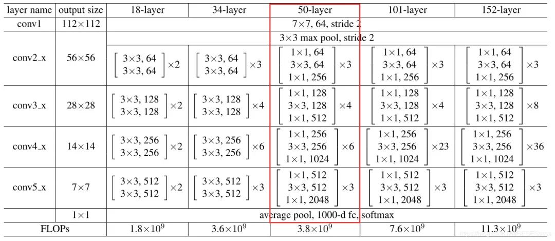
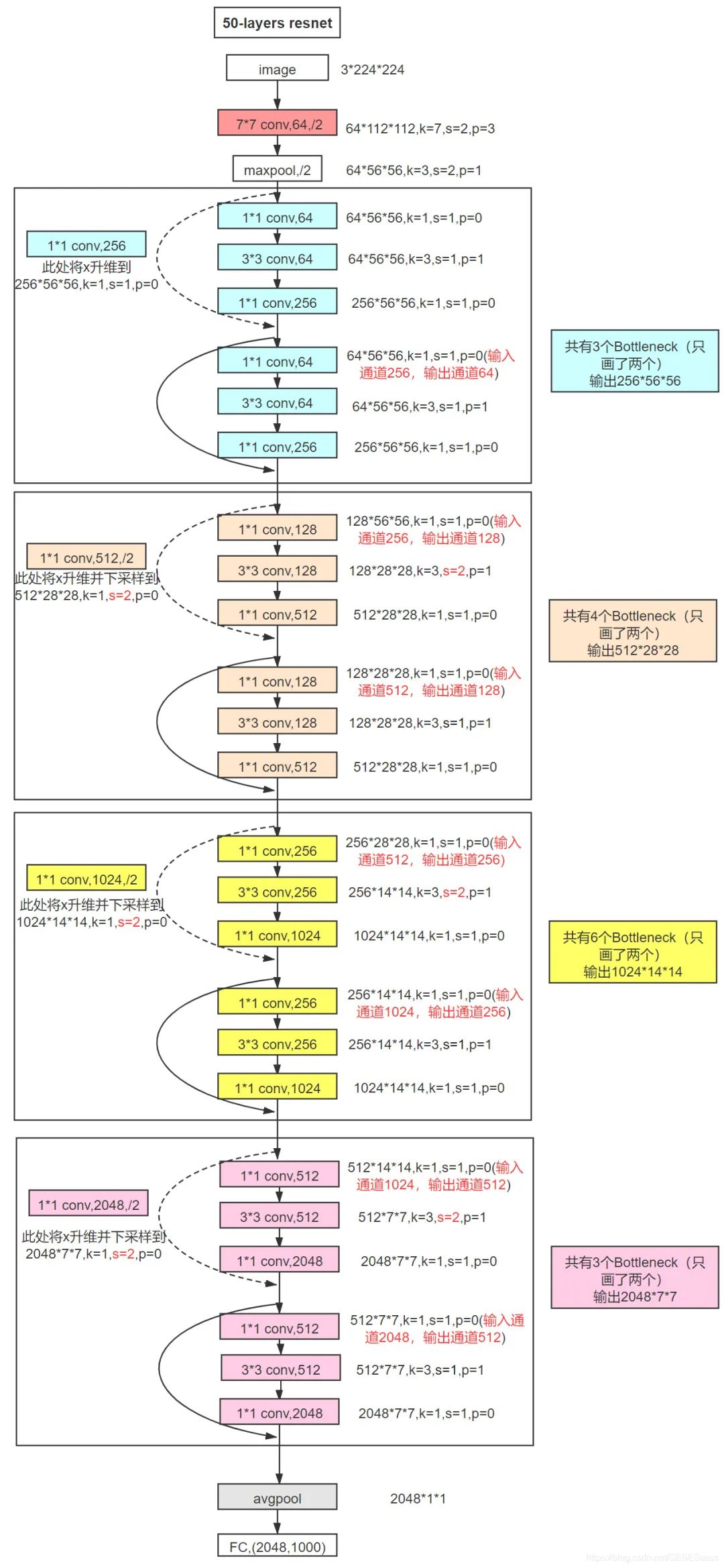
The paper divides ResNet-50 into four large convolution groups, each called a Bottleneck module (with more channels for input and output feature maps, while the convolution layers in the middle have a shallower feature depth, resembling a bottleneck structure). Bottleneck modules are connected via shortcut connections.
Left: Non-bottleneck structure, Right: Bottleneck structure
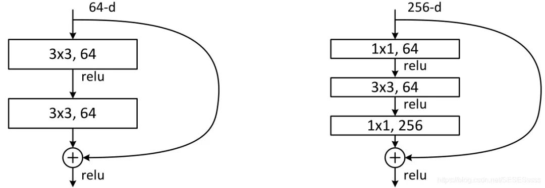
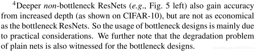
It is worth noting that ResNet uses the Bottleneck structure primarily to reduce the number of parameters in the network (feature dimensionality reduction), and in practice, the author noted that the use of bottleneck structures also encountered the degradation problem of ordinary networks:
3.2.3 ResNet-50 Diagram and Layer Parameter Details
For F(x)+x, ResNet adopts a channel-wise addition, so when adding, it is necessary to consider whether the number of channels is the same. If they are the same, they can be added directly (shown by the solid line in the figure). If the number of channels differs, a 1×1 convolution is needed to upscale the features to match the number of channels (shown by the dashed line in the figure):
3.2.4 Implementing a Bottleneck Module:
# Encapsulate Conv + BN into a basic convolution class:
class BasicConv2d(nn.Module):
    def __init__(self, in_channel, out_channel, kernel_size, stride=1, padding=0):
        super(BasicConv2d, self).__init__()
        self.conv = nn.Sequential(
            nn.Conv2d(in_channel, out_channel, kernel_size,
                      stride=stride, padding=padding, bias=False),
            nn.BatchNorm2d(out_channel)
        )

    def forward(self, x):
        x = self.conv(x)
        return x

# A Bottleneck module:
class Bottleneck(nn.Module):
    def __init__(self, in_channel, mid_channel, out_channel, stride=1):
        super(Bottleneck, self).__init__()

        self.judge = in_channel == out_channel

        self.bottleneck = nn.Sequential(
            BasicConv2d(in_channel, mid_channel, 1),
            nn.ReLU(True),
            BasicConv2d(mid_channel, mid_channel, 3, padding=1, stride=stride),
            nn.ReLU(True),
            BasicConv2d(mid_channel, out_channel, 1),
        )
        self.relu = nn.ReLU(True)
        # The downsampling part consists of a 1x1 convolution with a BN layer:
        if in_channel != out_channel:
            self.downsample = BasicConv2d(
                in_channel, out_channel, 1, stride=stride)

    def forward(self, x):
        out = self.bottleneck(x)
        # If the channels are inconsistent, downsample using a 1x1 convolution
        if not self.judge:
            self.identity = self.downsample(x)
            # Residual + identity mapping = output
            out += self.identity
        # Otherwise, add directly
        else:
            out += x

        out = self.relu(out)

        return out
3.2.5 Implementing ResNet-50
# ResNet50:
class ResNet_50(nn.Module):
    def __init__(self, class_num):
        super(ResNet_50, self).__init__()
        self.conv = BasicConv2d(3, 64, 7, stride=2, padding=3)
        self.maxpool = nn.MaxPool2d(3, stride=2, padding=1)
        # Convolution Group 1
        self.block1 = nn.Sequential(
            Bottleneck(64, 64, 256),
            Bottleneck(256, 64, 256),
            Bottleneck(256, 64, 256),
        )
        # Convolution Group 2
        self.block2 = nn.Sequential(
            Bottleneck(256, 128, 512, stride=2),
            Bottleneck(512, 128, 512),
            Bottleneck(512, 128, 512),
            Bottleneck(512, 128, 512),
        )
        # Convolution Group 3
        self.block3 = nn.Sequential(
            Bottleneck(512, 256, 1024, stride=2),
            Bottleneck(1024, 256, 1024),
            Bottleneck(1024, 256, 1024),
            Bottleneck(1024, 256, 1024),
            Bottleneck(1024, 256, 1024),
            Bottleneck(1024, 256, 1024),
        )
        # Convolution Group 4
        self.block4 = nn.Sequential(
            Bottleneck(1024, 512, 2048, stride=2),
            Bottleneck(2048, 512, 2048),
            Bottleneck(2048, 512, 2048),
        )
        self.avgpool = nn.AvgPool2d(4)
        self.classifier = nn.Linear(2048, class_num)

    def forward(self, x):
        x = self.conv(x)
        x = self.maxpool(x)
        x = self.block1(x)
        x = self.block2(x)
        x = self.block3(x)
        x = self.block4(x)
        x = self.avgpool(x)
        x = x.view(x.size(0), -1)
        out = self.classifier(x)

        return out
4.FPN (Feature Pyramid)
4.1 Semantic Information of Features
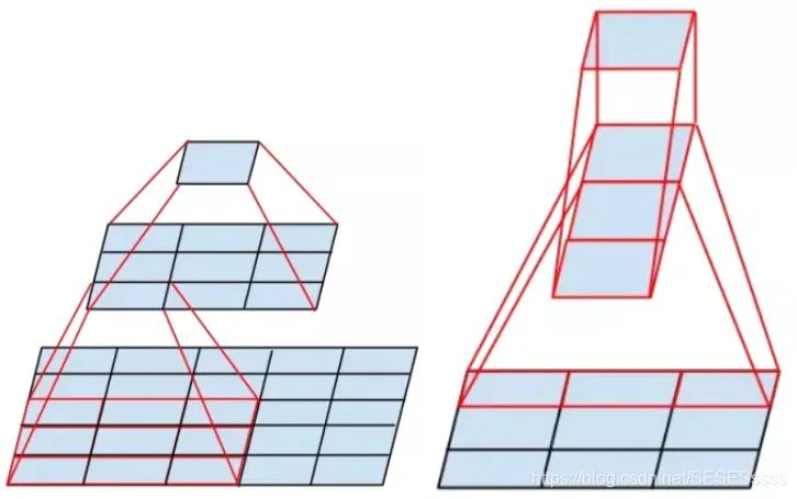
For CNN networks, images processed through the shallow convolution layers often output feature maps that only represent simple semantic information (like simple lines). The deeper the network, the more complex the semantic information extracted (from some textures to similar contours of certain categories): (The features in the figure have undergone deconvolution upsampling)
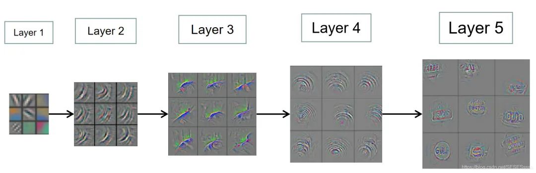
Therefore, traditional detection networks usually only use the high-level semantic feature maps from the last convolution output for subsequent steps, but this inevitably presents some problems.
4.2 Improvements
We know that the deeper the network, the higher the downsampling rate of features, meaning that a single pixel in deep feature maps corresponds to a region of shallow features. This does not significantly impact the detection of large targets. However, for small targets in the image, the effective information on deep features is limited, leading to a sharp decline in the network’s detection performance for small objects. This phenomenon is also known as the multi-scale problem.
To address the multi-scale problem, a straightforward solution is to use an image pyramid, transforming the original input into multiple images of different sizes, performing feature extraction on these images, and generating multi-scale features for subsequent processing. This way, the probability of detecting small targets on small-scale features is greatly increased. This method is simple and effective, and has been widely used in COCO object detection competitions. However, its drawback is the large computational load, requiring significant time.
In response, the FPN network (Feature Pyramid Networks) improved the method of extracting multi-scale features. Based on the introduction in 4.1, we know that the feature sizes extracted by different layers of the convolution network differ, resembling a pyramid structure. Additionally, the semantic information of each layer is also different; the shallower the features, the simpler the semantic information and the more details displayed, while the deeper the features, the less detail displayed and the higher the semantic information. Based on this, the FPN network integrates features from different convolution layers during the feature extraction process, effectively improving the multi-scale detection problem.
4.3 PyTorch Reproduction of FPN
4.3.1 FPN Network Architecture
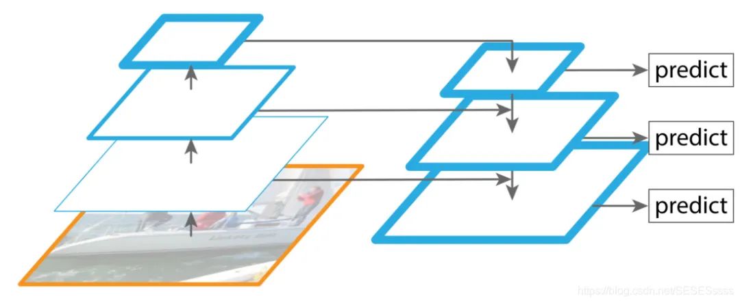
The FPN network mainly consists of four parts: bottom-up network, top-down network, lateral connections, and convolution fusion.

-
Bottom-up Network (providing features of different scales):
On the far left is a regular feature extraction convolution network (ResNet), where C2-C4 represents four large convolution groups in ResNet, each containing multiple Bottleneck structures. The input of the original image starts from this structure.
-
Top-down Network (providing high-level semantic features): In this structure, first, a 1×1 convolution is applied to C5 to reduce the channel count to obtain M5, and then upsampling is sequentially performed to obtain M4, M3, and M2. The goal is to obtain features of the same size as C4, C3, and C2 but with different semantics, facilitating feature fusion (the fusion method is element-wise addition).
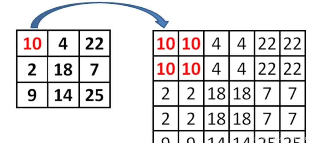
It is worth noting that during the upsampling process of the network, the method used is not deconvolution or non-linear interpolation, but regular nearest-neighbor upsampling (which can preserve the semantic information of the feature map to the greatest extent, resulting in features that have good spatial information and strong semantic information): 【Paper Notes】 FPN — Feature Pyramid: https://zhuanlan.zhihu.com/p/92005927
-
Lateral Connections:
Fuse high-level semantic features with shallow detail features (using 1×1 convolutions to ensure that the number of channels is the same).
-
Convolution Fusion:
After obtaining the added features, further fuse M2-M4 using 3×3 convolutions (the paper states that this can eliminate the overlapping effect caused by upsampling).
4.3.2 Reproducing the FPN Network
# Import resnet50
resnet = models.resnet50(pretrained=True)
# Split into blocks to extract features from different depth networks
layer1 = nn.Sequential(
    resnet.conv1,
    resnet.bn1,
    resnet.relu,
    resnet.maxpool,
)
layer2 = resnet.layer1
layer3 = resnet.layer2
layer4 = resnet.layer3
layer5 = resnet.layer4


class FPN(nn.Module):
    def __init__(self):
        super(FPN, self).__init__()
        # 3x3 convolution for feature fusion
        self.MtoP = nn.Conv2d(256, 256, 3, 1, 1)
        # Lateral connections, using 1x1 convolution for dimensionality reduction
        self.C2toM2 = nn.Conv2d(256, 256, 1, 1, 0)
        self.C3toM3 = nn.Conv2d(512, 256, 1, 1, 0)
        self.C4toM4 = nn.Conv2d(1024, 256, 1, 1, 0)
        self.C5toM5 = nn.Conv2d(2048, 256, 1, 1, 0)
    # Feature fusion method
    def _upsample_add(self, in_C, in_M):
        H = in_M.shape[2]
        W = in_M.shape[3]
        # Nearest neighbor upsampling method
        return F.upsample_bilinear(in_C, size=(H, W)) + in_M

    def forward(self, x):
        # Bottom-up
        C1 = layer1(x)
        C2 = layer2(C1)
        C3 = layer3(C2)
        C4 = layer4(C3)
        C5 = layer5(C4)
        # Top-down + lateral connections
        M5 = self.C5toM5(C5)
        M4 = self._upsample_add(M5, self.C4toM4(C4))
        M3 = self._upsample_add(M4, self.C3toM3(C3))
        M2 = self._upsample_add(M3, self.C2toM2(C2))
        # Convolution fusion
        P5 = self.MtoP(M5)
        P4 = self.MtoP(M4)
        P3 = self.MtoP(M3)
        P2 = self.MtoP(M2)
        # Returns multi-scale features
        return P2, P3, P4, P5
Good news!
Beginner Learning Vision Knowledge Circle
Is now open to the public👇👇👇
Download 1: Chinese Tutorial for OpenCV-Contrib Extension Modules
Reply "Chinese Tutorial for Extension Modules" in the background of the "Beginner Learning Vision" public account to download the first Chinese tutorial for OpenCV extension modules on the internet, covering installation of extension modules, SFM algorithms, stereo vision, target tracking, biological vision, super-resolution processing, and more than twenty chapters of content.

Download 2: 52 Lectures on Python Vision Practical Projects
Reply "Python Vision Practical Projects" in the background of the "Beginner Learning Vision" public account to download 31 visual practical projects including image segmentation, mask detection, lane line detection, vehicle counting, eye line addition, license plate recognition, character recognition, emotion detection, text content extraction, face recognition, etc., to assist in quickly learning computer vision.

Download 3: 20 Lectures on OpenCV Practical Projects
Reply "20 Lectures on OpenCV Practical Projects" in the background of the "Beginner Learning Vision" public account to download 20 practical projects based on OpenCV to advance your OpenCV learning.

Group Chat

Welcome to join the reader group of the public account to communicate with peers. There are currently WeChat groups for SLAM, 3D vision, sensors, autonomous driving, computational photography, detection, segmentation, recognition, medical imaging, GAN, algorithm competitions, etc. (these will gradually be subdivided in the future). Please scan the WeChat ID below to join the group, and note: "Nickname + School/Company + Research Direction", for example: "Zhang San + Shanghai Jiao Tong University + Vision SLAM". Please follow the format, otherwise, you will not be approved. After successful addition, you will be invited to the relevant WeChat group based on your research direction. Please do not send advertisements in the group, or you will be removed. Thank you for your understanding~