Network representation learning (network embedding) has emerged in recent years as a branch of feature learning research.

As a dimensionality reduction method, network representation learning aims to map the nodes in a network into a low-dimensional continuous vector space while preserving the structure information of the original network in that low-dimensional space, aiding subsequent tasks such as link prediction, node classification, recommendation systems, clustering, and visualization.

In this PhD Talk, Wang Hongwei from Shanghai Jiao Tong University reviewed the research progress in the field of network representation learning over the past five years.

He then interpreted, as the first author, the work published by Shanghai Jiao Tong University, Microsoft Research Asia, and the Hong Kong Polytechnic University at AAAI 2018: GraphGAN: Graph Representation Learning with Generative Adversarial Nets. This work introduces the framework of Generative Adversarial Networks (GAN) to perform network feature learning through adversarial training between a generator and a discriminator.

Finally, he briefly introduced the applications of network representation learning in sentiment prediction and recommendation systems, which are his latest results published as the first author in top international conferences on data mining such as WSDM, CIKM, and WWW.

△ Talk replay

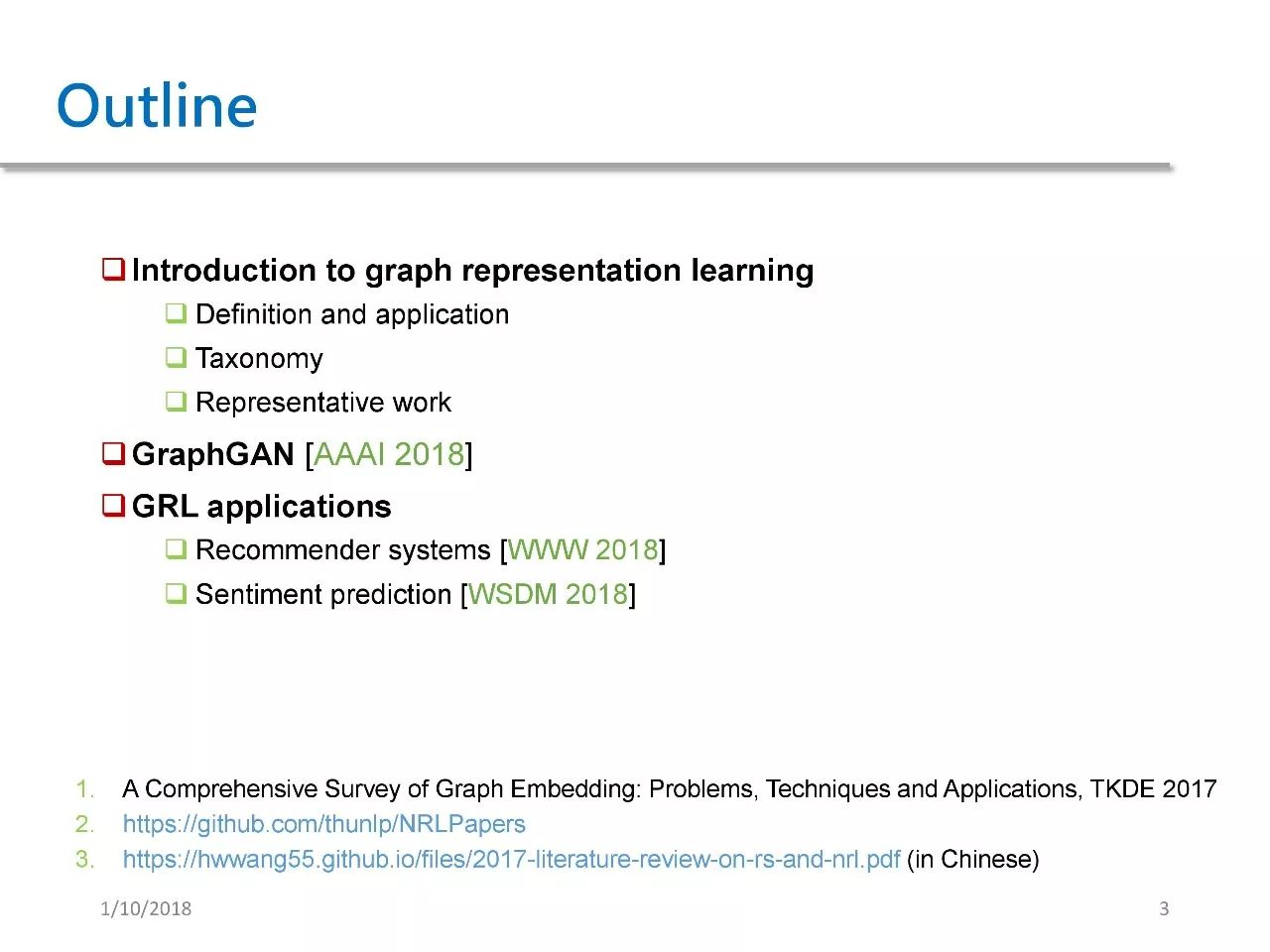
This live broadcast is mainly divided into three parts. First, I will introduce the definition, applications, classification methods, and related representative works of Graph Representation Learning.

In the second part, I will introduce our paper published at AAAI 2018 GraphGAN: Graph Representation Learning with Generative Adversarial Nets.

Finally, I will introduce some applications of Graph Representation Learning, including recommendation and sentiment prediction.

The bottom of the above image shows three valuable resources: the first is a Survey on Graph Embedding, the second is a paper list that includes classic papers related to Network Representation Learning from the past five years. The third is a literature review on recommendation systems and network representation learning that I authored, welcome to refer.

About GRL

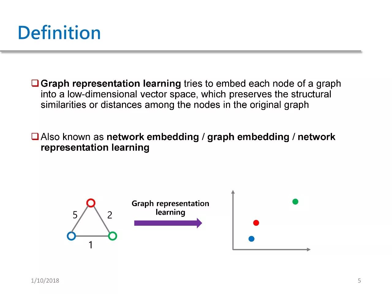
First, let me briefly introduce the definition of Graph Representation Learning, which can be termed as graph feature learning or network feature learning in Chinese. Its main purpose is to map each node in the graph to a low-dimensional vector space while preserving the original graph’s structural or distance information within this space.

This is not an official authoritative definition; Graph Representation Learning currently has no official definition or name, and it can also be referred to as Network Embedding, Graph Embedding, or GRL.

Let’s look at a simple example in the above image. The left graph has three nodes and three edges, with the numbers indicating the weights of each edge. We map it to a two-dimensional space through GRL. It can be observed that the greater the weight between two points, the closer their distance in the low-dimensional space. This is the essence of GRL, which is to preserve the original graph’s structural information in the low-dimensional space.

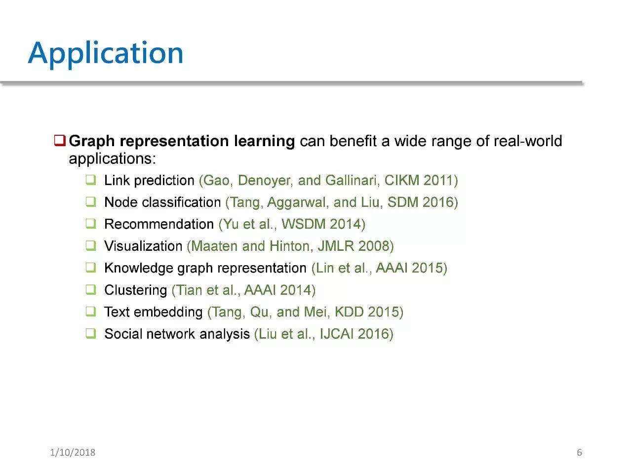
Graph Representation Learning has a wide range of applications. It can be used for link prediction, node classification, recommendation systems, visualization, knowledge graph representation, clustering, Text Embedding, and social network analysis.

GRL Classification Methods

We will briefly introduce GRL methods classified into three different categories.

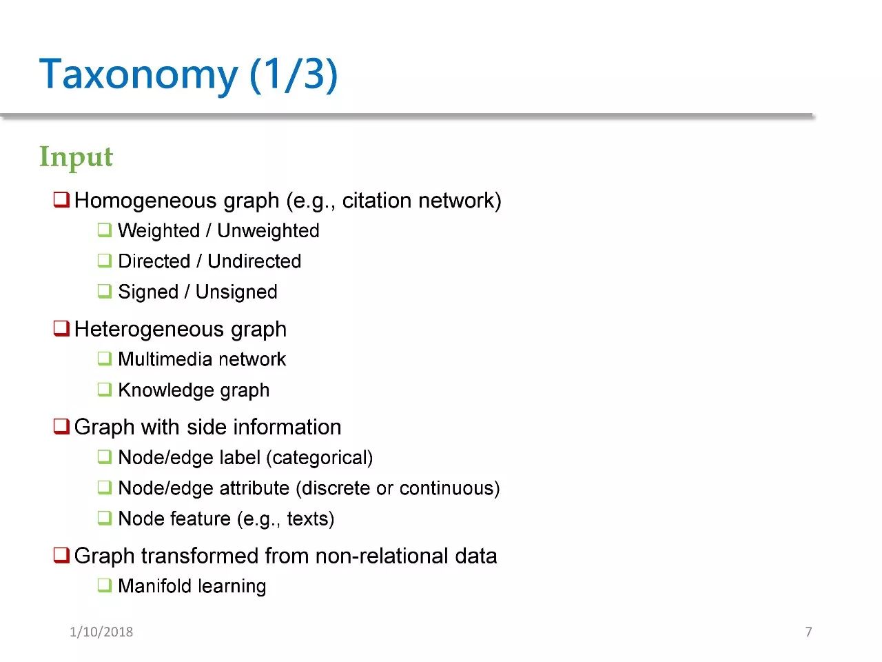
First, classification by input. Since it is GRL, the input must be a graph, but there are many types of graphs:

The first type is homogeneous graphs, where nodes and edges are of only one type, such as citation networks, where nodes represent each paper, and edges represent citation relationships. Homogeneous graphs can be further subdivided based on whether they are weighted, directed, or have positive or negative weights.

The second type is heterogeneous graphs, where nodes and edges are of multiple types, generally divided into two situations:

1. Multimedia networks. For example, some papers have considered a graph with image and text as two types of nodes, and three types of edges: image-text, image-image, and text-text.

2. Knowledge graphs. The nodes in the graph represent entities, and edges represent relationships. Each triple, HRT, indicates that the head node H and tail node T have a relationship R. Since relationship R can take many forms, KG also belongs to a type of heterogeneous graph.

The third type is Graph with side information, where side information refers to auxiliary information. This type of graph indicates that besides edges and nodes, both nodes and edges carry auxiliary information, such as labels for edges and nodes, or attributes for edges and nodes, or nodes having features.

The differences lie in that labels are categorical, attributes can be discrete or continuous, while features may include text or images and other more complex characteristics.

The fourth type is Graph Transformed from non-relational data, which refers to graphs converted from non-relational data, usually indicating some data in high-dimensional space. This is typically the type of data used in early GRL methods, with the most typical example being manifold learning, which we can understand as a dimensionality reduction method.

We can also classify GRL methods based on output content.

The first method outputs node embeddings, which means outputting an embedding for each node, and this is the most common output. Most of the methods mentioned earlier basically output node embeddings.

The second method outputs edge embeddings, which means outputting an embedding for each edge. This output has two cases; one is in KG, where we output for each relation, that is, each edge. In link prediction applications, we also output a feature for each edge and use it as edge features for classification tasks in subsequent work.

The third method outputs sub-graph embeddings, which means the embedding of subgraphs, including embeddings of substructures or communities.

The fourth is the embedding of the entire graph, which means outputting an embedding for the entire graph. If we perform embedding on proteins or molecules which are numerous small graphs, we can compare the similarity between two molecules.

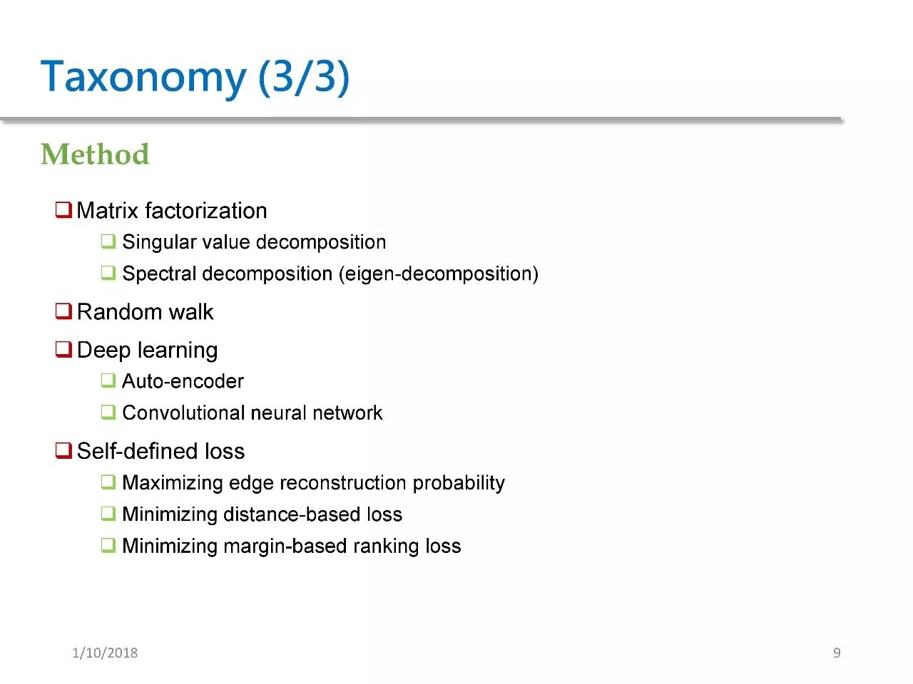
The third classification method is based on the approach.

The first method is based on matrix decomposition. Generally, matrix decomposition includes singular value decomposition and spectral decomposition; spectral decomposition is what we commonly refer to as feature decomposition, which is a traditional method.

The second method is based on random walks. This method is well-known, and the Deep Walk we will mention later is based on random walks.

The third method is based on deep learning. This includes methods based on autoencoders and convolutional neural networks.

The fourth method is based on some custom loss functions. This includes three situations: the first is to maximize edge reconstruction probability, the second is to minimize distance-based loss functions, and the third is to minimize margin-based ranking loss, which is common in KG embedding.

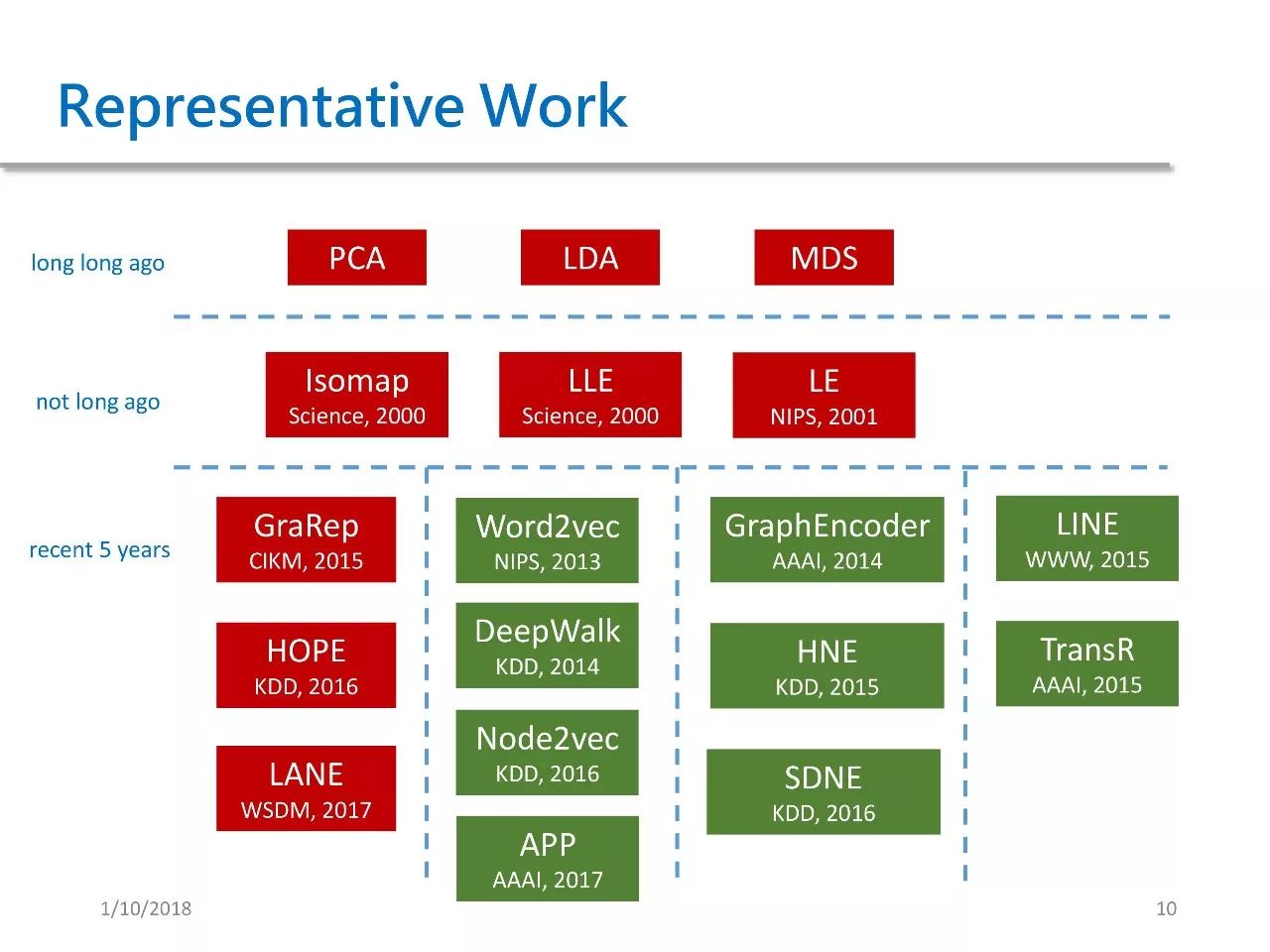
The image above shows the representative works of GRL methods. They can be divided into three categories chronologically: the first category includes traditional methods, including PCA, LDA, MDS, and other dimensionality reduction methods.

A batch of classic methods appeared around the year 2000, including ISOMAP isometric mapping, LLE local linear embedding, and LE Laplacian eigenmap.

Many methods have also been proposed in the last five years, which I have categorized into four types, each corresponding to the aforementioned classification based on methods.

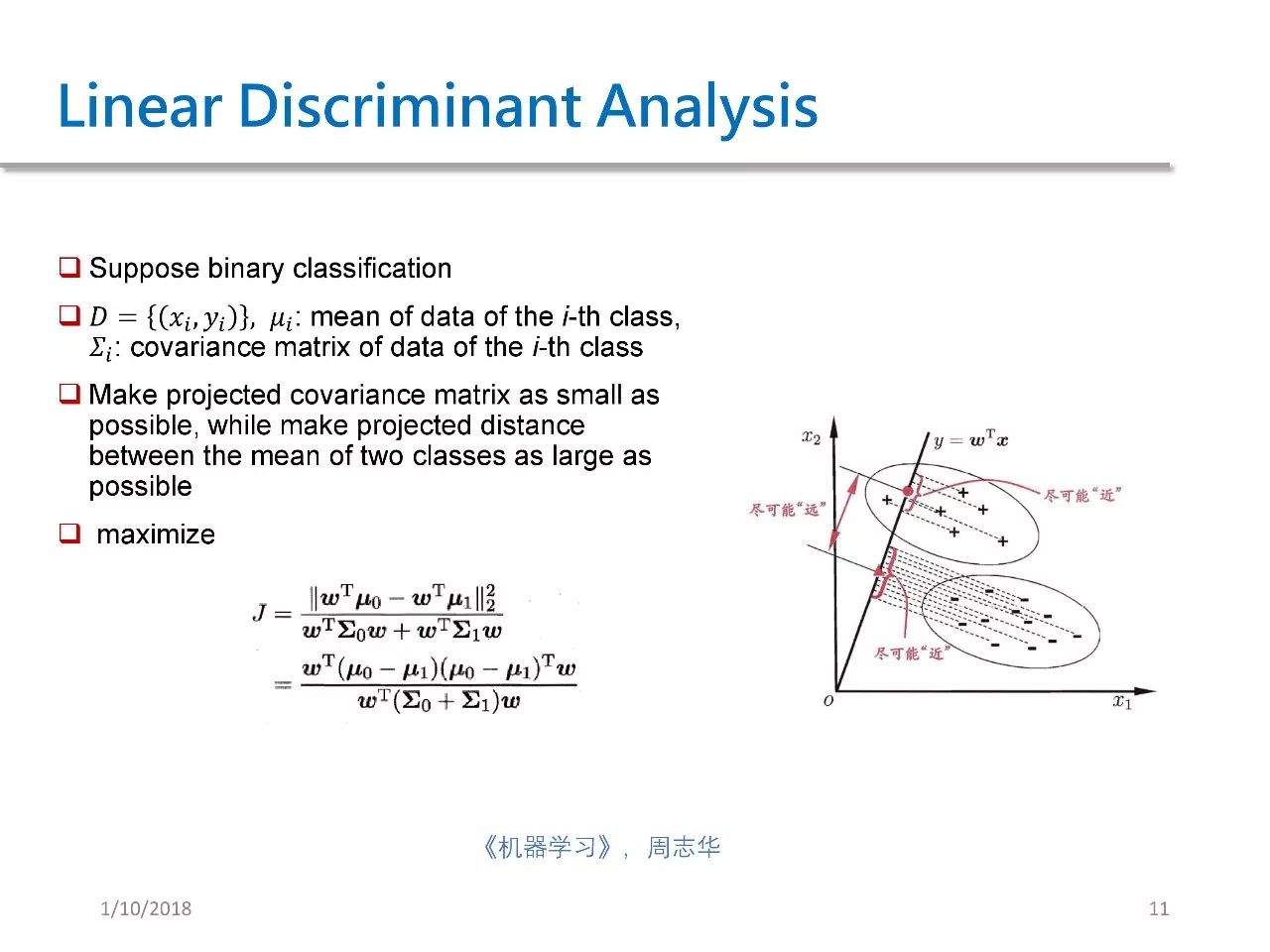
LDA Linear Discriminant Analysis is a traditional supervised dimensionality reduction method. In the right image, there are two types of points, one represented by positive signs and the other by negative signs.

We need to map the two-dimensional points to one dimension, and the goal of LDA is to make the projected points of the same class as close as possible, i.e., to minimize their covariance, while maximizing the distance between points of different classes.Only in this way can it classify or cluster these points in low-dimensional space.

Locally Linear Embedding is a typical manifold learning method, which refers to mapping input from high-dimensional space to low-dimensional space while preserving the linear dependencies among neighbors in the low-dimensional space.

The lower left image is a typical example of manifold learning, where the manifold refers to existing low-dimensional structures in high-dimensional space; for example, Graph A looks like a Swiss roll, which is a typical two-dimensional structure in three-dimensional space. Through LLE, we can unfold it into a two-dimensional structure.

The purpose of this method is to preserve neighbor information in high-dimensional space. The specific approach is as follows: for each point Xi, we first need to determine its neighbor set, and then calculate parameters like Wik Wij. These parameters indicate that I want to use these neighbors to reconstruct Xi, which will have a unique analytical solution. After obtaining the W parameters, we then constrain in low-dimensional space using W to learn a low-dimensional embedding.

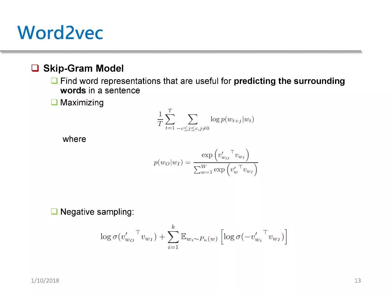
The essence of Word2vec is actually word embedding, not network embedding. However, due to its profound influence on subsequent network embedding methods, we will briefly introduce it.

Word2vec includes a skip-gram model, whose essence is to obtain a feature for each word and use this feature to predict surrounding words. Therefore, its specific method is to maximize the probability. This probability refers to the probability of each word in the window of T around a given center word WT.

This probability is actually computed using softmax. Due to the high cost of softmax, we usually use negative sampling as a substitute. Negative sampling refers to selecting some negative samples from the entire vocabulary for each word and treating them as negative samples.

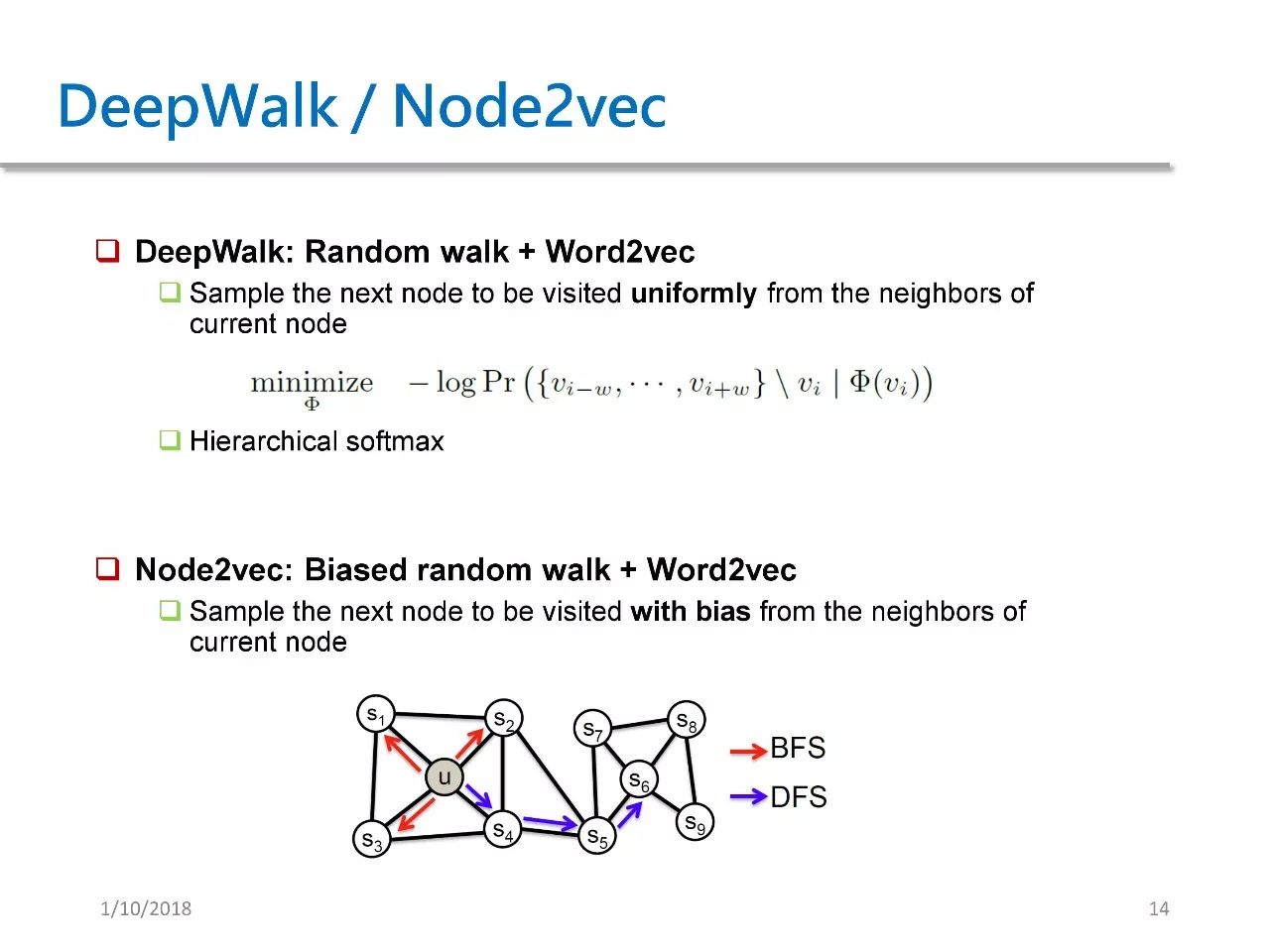
In Network Embedding, there are two typical works, DeepWalk and Node2vec. These two works were published in KDD 14 and KDD 16 respectively.

DeepWalk is equivalent to random walk + word2vec. Starting from each node in the graph, we perform random walks, uniformly and randomly selecting the next node, and then uniformly and randomly selecting the next node from the next node.

After repeating this N times, we obtain a path that can be treated as a sentence. This way, the problem is completely transformed into the domain of Word2vec.

You may ask, isn’t this method very simple? Isn’t it just applying Word2vec to network embedding?

Yes, it is that simple. Sometimes research does not emphasize how novel your method is or how sophisticated the mathematics is, but whether you can propose a method with a strong motivation and quick action.

Node2vec improves upon DeepWalk. It changes the original random walk to a biased random walk.

In DeepWalk, we uniformly select the next node. But in Node2vec, we select the next node non-uniformly. We can choose to mimic DFS and keep going deeper into the graph, or to mimic BFS and circle around a point.Thus, Node2vec is simply a minor improvement over DeepWalk.

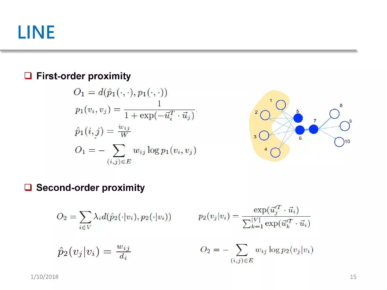
LINE stands for Large-scale Network Information Embedding. This paper was published in WWW 15. This work belongs to the custom loss functions we mentioned earlier because it defines two types of loss functions: one for first-order proximity and another for second-order proximity.

The so-called first-order proximity refers to whether two points are directly connected. In the right image, we can see that there is an edge connecting point six and point seven, which means they have a first-order proximity.

The second-order relationship refers to the similarity of the neighbors of two points. In the right image, points five and six are not directly connected, but their neighbors are completely overlapping, so we can consider that points five and six have a strong second-order proximity. Based on this proximity, LINE defines two loss functions O1 and O2, and then learns network embedding based on these two loss functions.

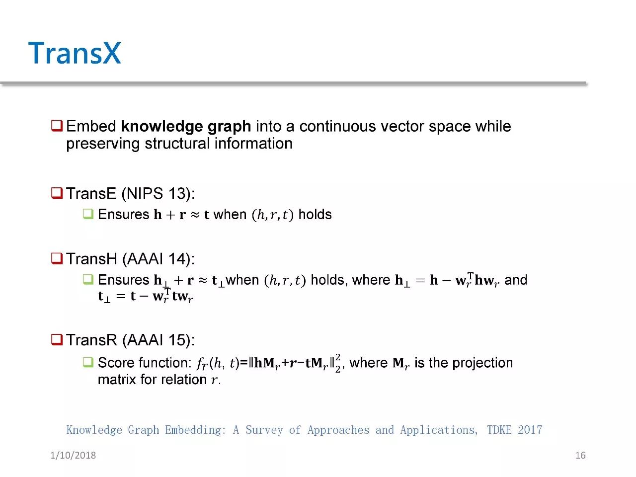
TransX represents a series of methods, where X can refer to any letter, and these methods are based on KG embedding. KG embedding refers to mapping each entity and relation in KG to a low-dimensional continuous space while preserving the original graph structure information.Classic methods include TransE, TransH, and TransR, collectively referred to as translation-based methods.

TransE has a very simple idea, which is to force the Head Embedding + relation embedding = tail embedding. In other words, it translates head plus relation into tail. Since this paper was published in NIPS 13, it has led to a wave of TransX methods. You can refer to the survey at the bottom of the above image, which includes at least about ten papers.

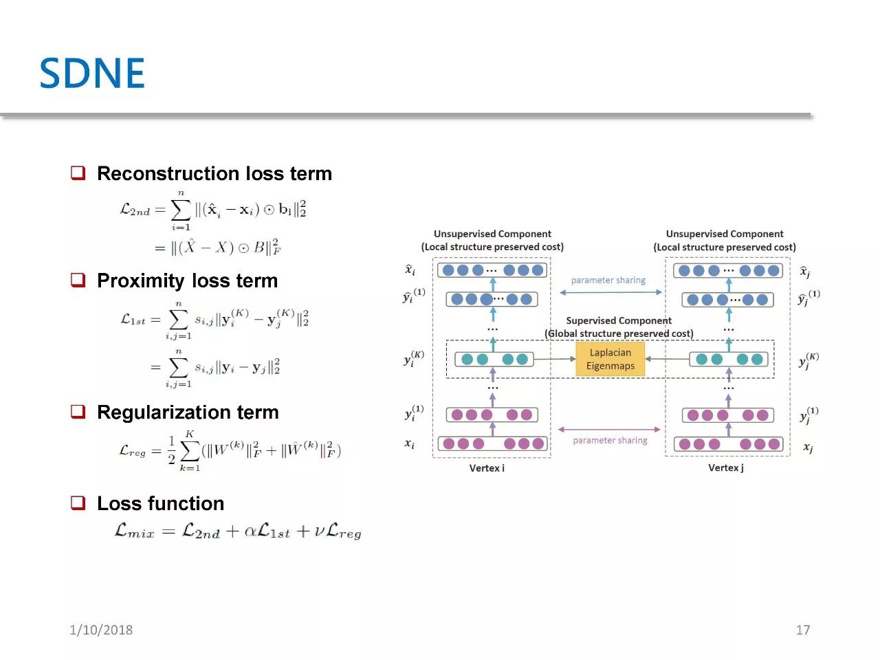
The last one is SDNE, which stands for Structured Deep Network Embedding. This paper was published in KDD 15, and its essence is a network embedding based on autoencoders.

Although the right image looks complex, its idea is very simple. The author designed an autoencoder whose input is the adjacency vector of each point.

There are three loss components: the first is reconstruction loss, the second is proximity loss term, which means that if two nodes are connected by an edge, their embeddings must be as close as possible, with the degree of closeness depending on their weights. The greater the weight, the greater the penalty for this loss. The third component is a regularization term.

GraphGAN

Earlier, we categorized Network Embedding methods into three classes, while in GraphGAN we divide them into two categories: the first is generative models, and the second is discriminative models.

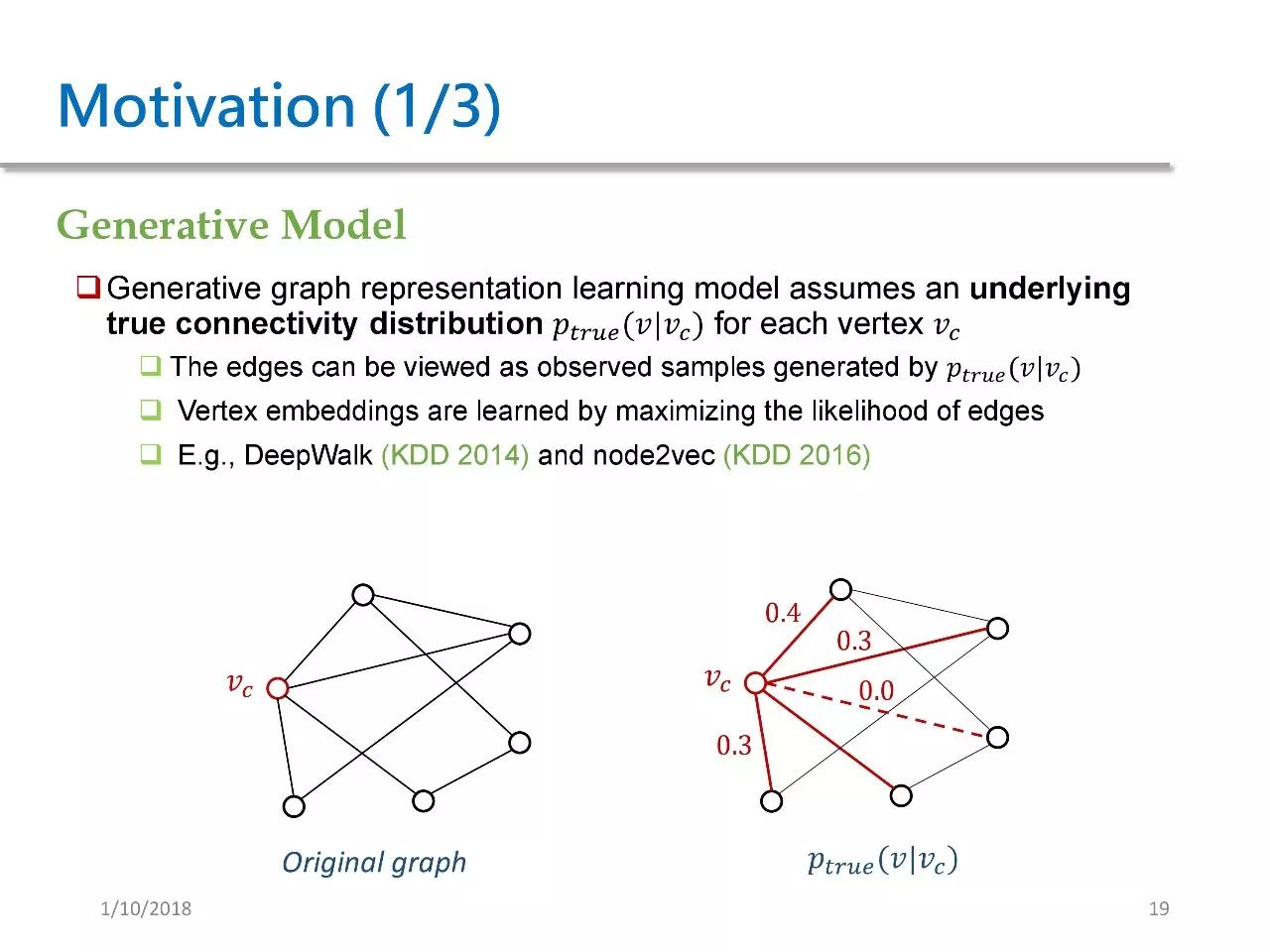
Generative models assume that there exists a latent, true continuous distribution Ptrue(V|Vc) in the graph. For a given Vc, we can see that Vc is connected to four nodes, and besides Vc, there are five other nodes. Ptrue(V|Vc) indicates the distribution over the other nodes except for Vc.

Assuming that there is such a distribution for each Vc in the graph, each edge in the graph can be viewed as samples drawn from Ptrue. These methods aim to maximize the likelihood of the edges to learn vertex embeddings. The previously mentioned DeepWalk and Node2vec belong to generative models.

Discriminative models attempt to learn the probability of an edge existing between two nodes directly. This method combines Vi and Vj as features and outputs the probability of the edge P(edge|Vi, Vj). The representative works of this method are SDNE and a PPNE paper presented at DASFAA.

After this classification, a natural idea arises: can the discriminative and generative models be combined? These two can actually be seen as two sides of a coin; they are opposing yet interconnected.

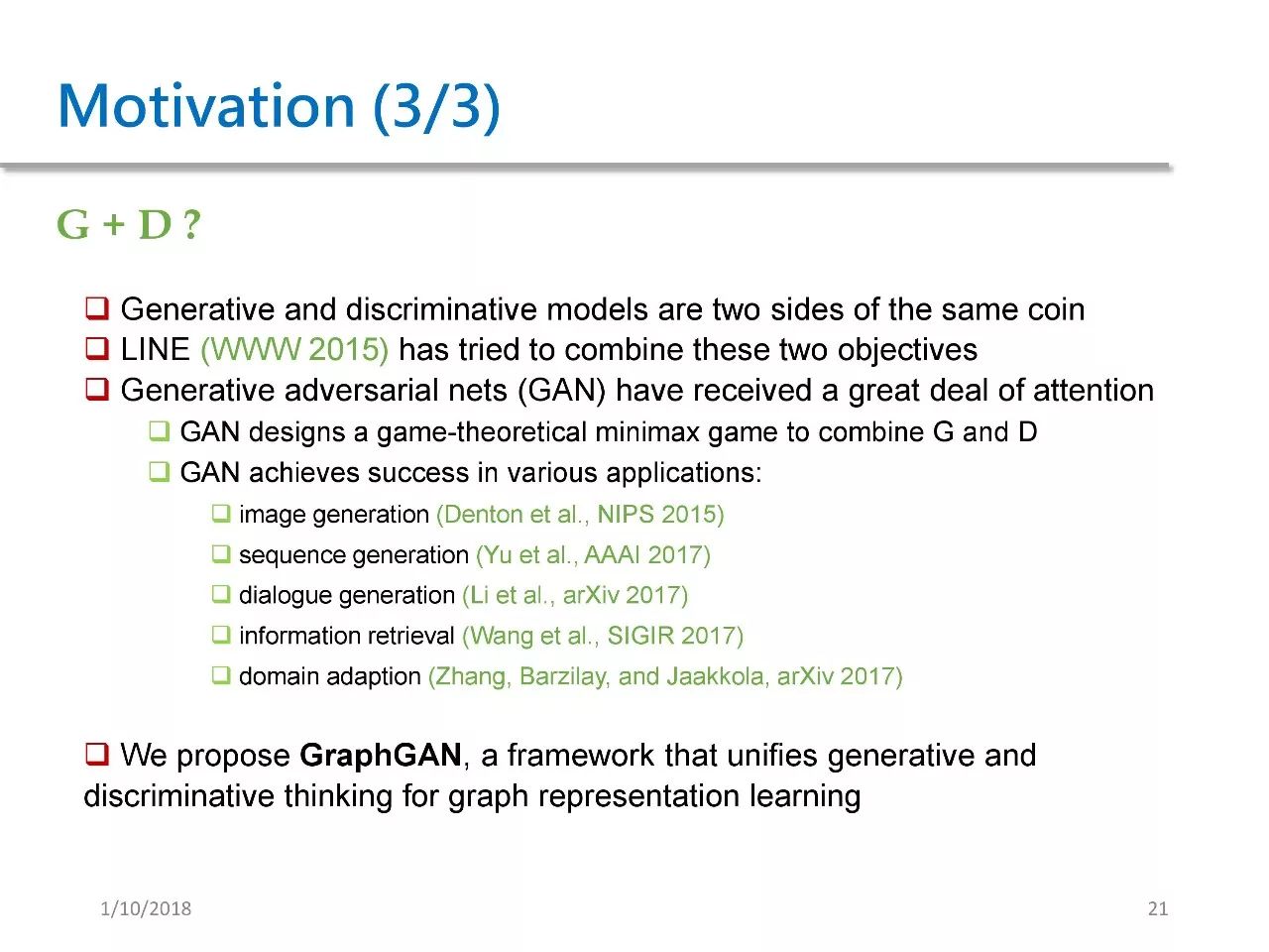
The LINE mentioned earlier has already attempted this. The first-order and second-order relationships mentioned in the text are actually different objective functions of the two models.

Generative adversarial networks have gained much attention since 2014; they define a game-theoretical minimax game that combines generative and discriminative models, achieving great success in applications such as image generation, sequence generation, dialogue generation, information retrieval, and domain adaptation.

Inspired by the above work, we proposed GraphGAN, which is a framework that combines generative and discriminative models in network generation learning.

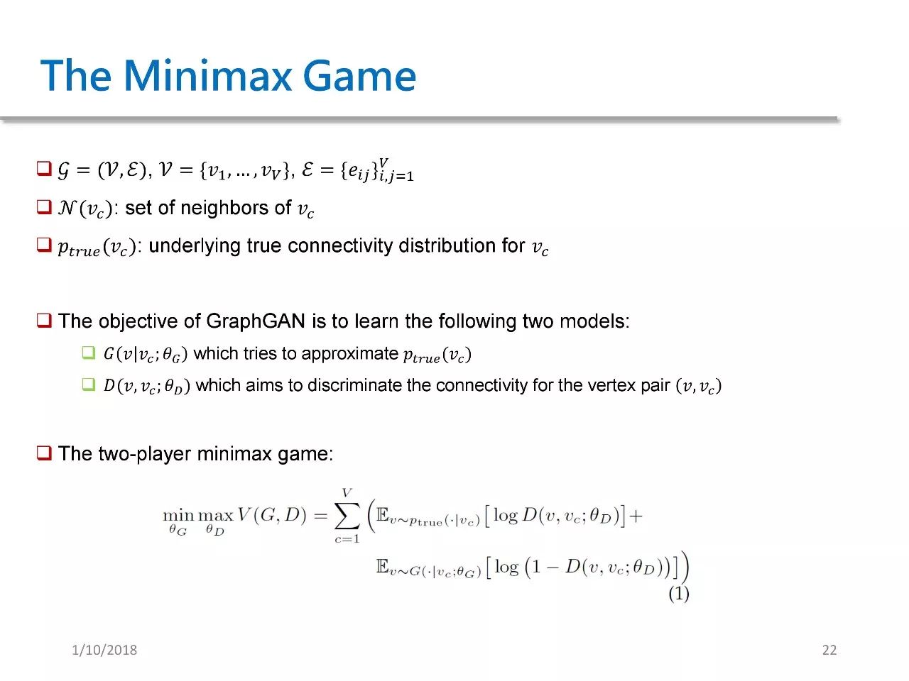
Next, I will introduce the Minimax Game. Here, V is the set of nodes, and E is the set of edges. We define N (Vc) as all neighbors of Vc in the graph and define Ptrue (Vc) as the true continuous distribution of Vc.

GraphGAN attempts to learn the following two models: the first is G(V|Vc), which tries to approach Ptrue (Vc). The second is D(V|Vc), which aims to determine whether there is an edge between V and Vc.

Thus, we obtain a two-player minimax game. This formula is the key to this article; only by fully understanding this formula can we continue to comprehend the following.

In this formula, we perform a minimax operation. Given θD, we attempt to minimize it, which is essentially summing the two expectations for each node in the graph.

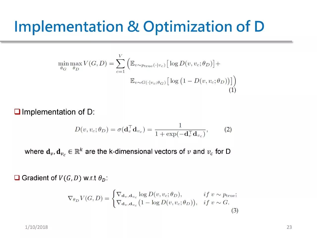
Next, let’s look at the implementation and optimization of the generator. In GraphGAN, we chose a very simple generator; the generator D(V, VC) is a sigmoid function that first computes the inner product of the embeddings of both, then processes it with the sigmoid function. The gradient for this implementation is naturally simpler.

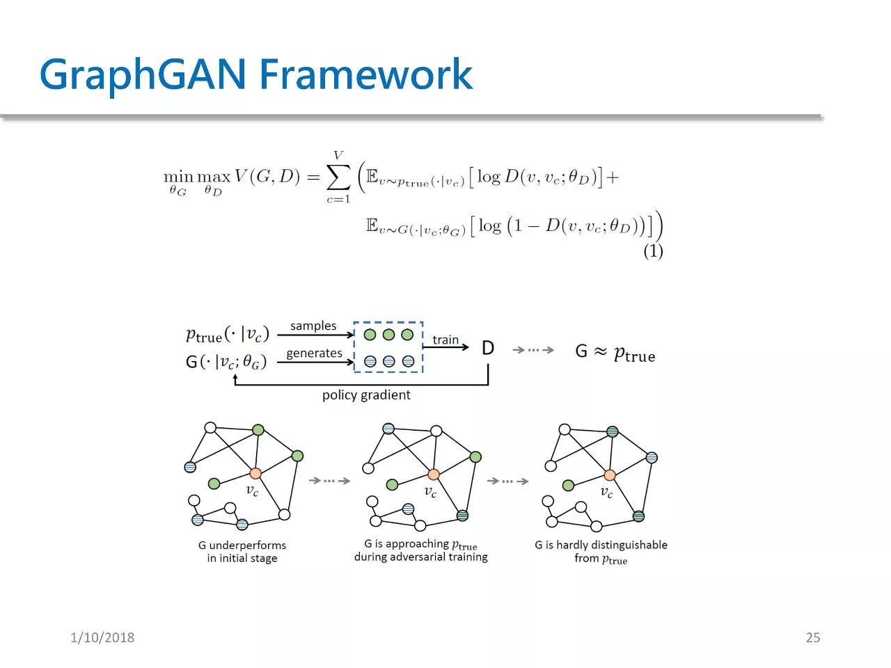
From the above image, we can see that in each iteration, we sample some green points that are truly adjacent to Vc from Ptrue, and then generate some blue points that are connected to Vc from G. We treat the green points as positive samples and the blue points as negative samples to train D. After obtaining D, we use the signals from D to train G.

This is the policy gradient process mentioned earlier. We continuously repeat this process until the generator G and Ptrue are very close.

At the beginning, G is relatively poor, so for a given Vc, the points sampled by G are far from Vc. As training progresses, the sampled points by G will gradually approach Vc, and eventually, the sampled points by G will almost all become truly adjacent to Vc, making G and Ptrue difficult to distinguish.

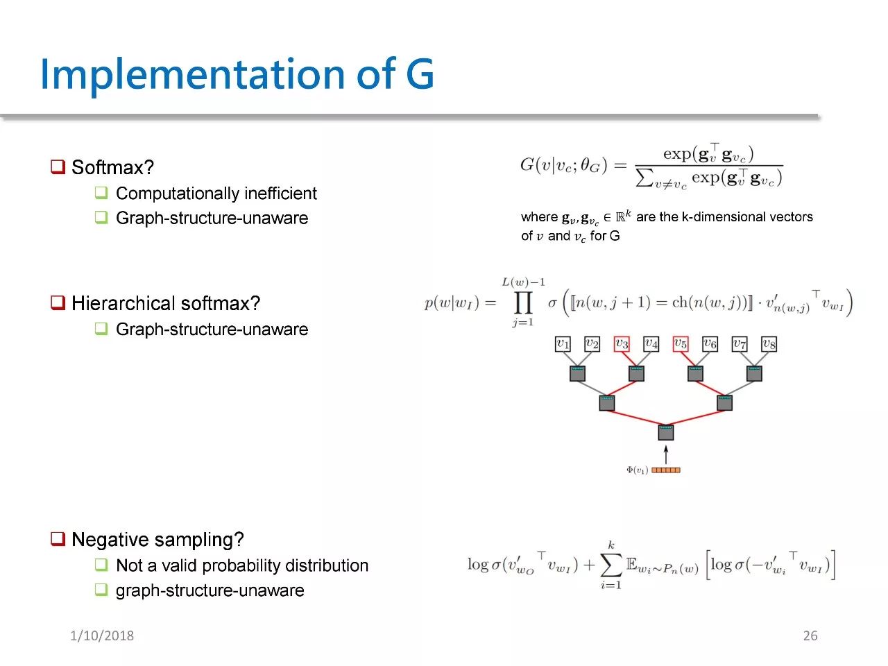
Next, we will discuss the implementation of G. One intuitive idea is to use softmax to implement G, defining G(v|VC) as a softmax function.

This definition has two problems: first, the computational complexity is too high, as it involves all nodes in the graph, and the derivatives also need to update all nodes in the graph. This makes it difficult to apply to large-scale graphs. The second problem is that it does not consider the structural characteristics of the graph, meaning the distances of these points from Vc are not taken into account.

The second method is to use hierarchical softmax, specifically organizing a binary tree and placing all nodes at the leaf positions, then calculating the current Vc from the root. Since there is a unique path from the root to each leaf node, this computation can be converted to a calculation along the path in the tree, resulting in a computational complexity of logN, where N represents the depth of the tree. Although this approach simplifies the calculation, it still does not account for the structural characteristics of the graph.

The third method is Negative Sampling. This method is actually an optimization method; it does not produce an effective probability distribution and similarly does not consider the structural feature information of the graph.

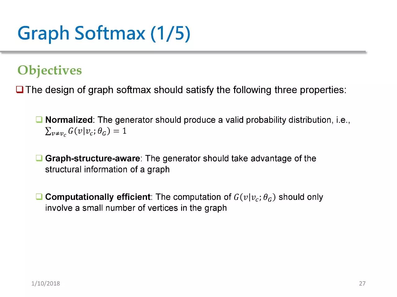
In GraphGAN, our goal is to design a softmax method that satisfies the following three requirements. The first requirement is regularization, meaning the probabilities sum to 1; it must be a valid probability distribution. The second requirement is that it should be able to perceive the graph structure and fully utilize the structural feature information of the graph. Finally, the third requirement is high computational efficiency, meaning the G probabilities should only involve a small subset of nodes in the graph.

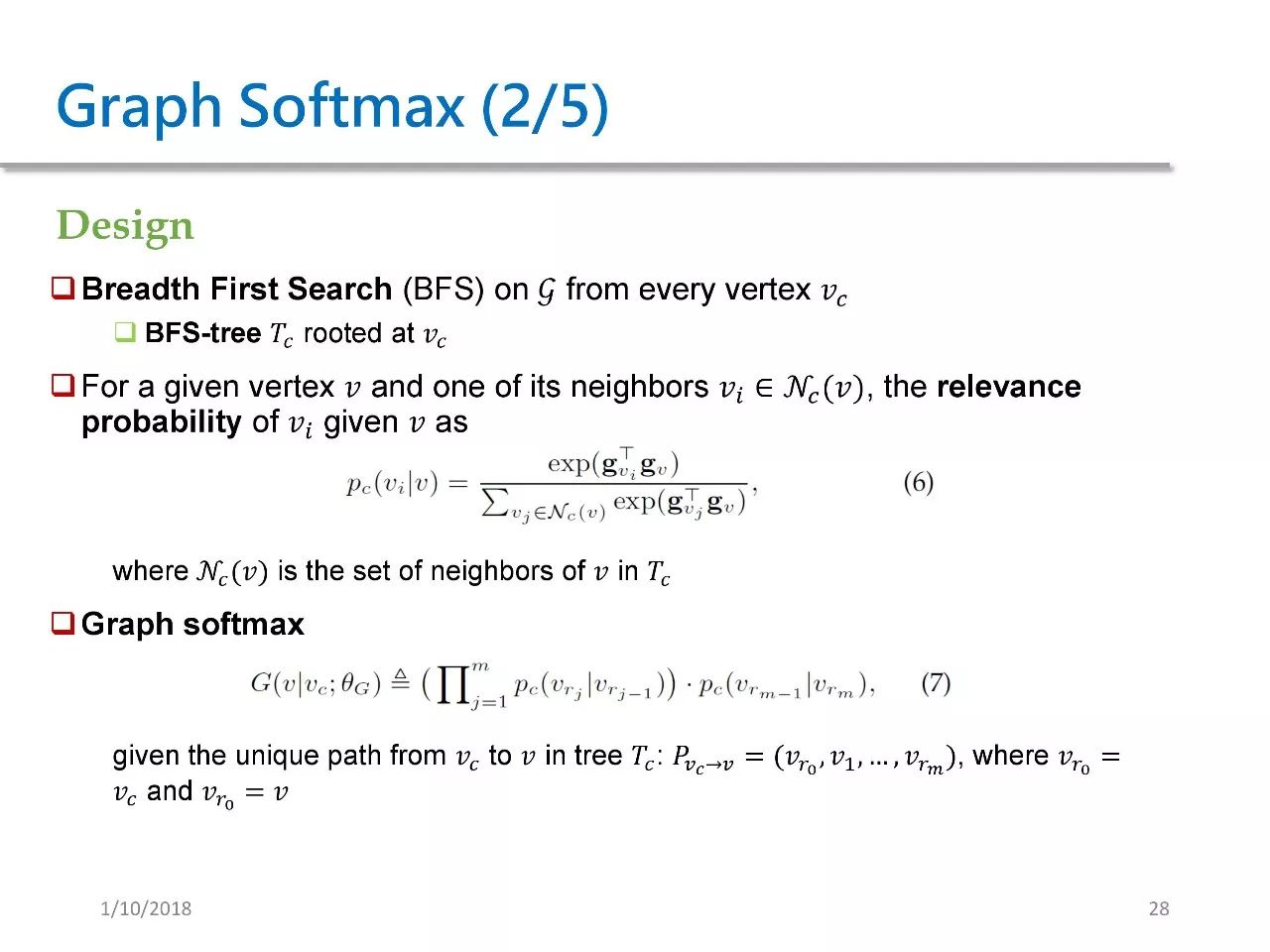
For each given node Vc, we need to perform a BFS (Breadth-First Search) starting from Vc to obtain a BFS tree rooted at Vc. For each node in this tree, we define a relevance probability. In fact, this is a softmax over the neighbors of Vc.

We can prove the following three properties:

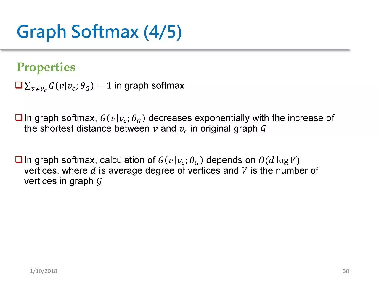
1. The probability of graph softmax sums to 1;

2. In graph softmax, the farther apart two nodes are in the original graph, the lower their probability; this fully utilizes the structural characteristics of the graph, as the farther the shortest distance between two nodes in the original graph, the lower the probability of an edge existing between them;

3. In the computation of graph softmax, the calculation only depends on O(d log V). d is the average degree of each node in the graph, and V is the size of the nodes in graph G. This number will be significantly smaller than the complexity of softmax.

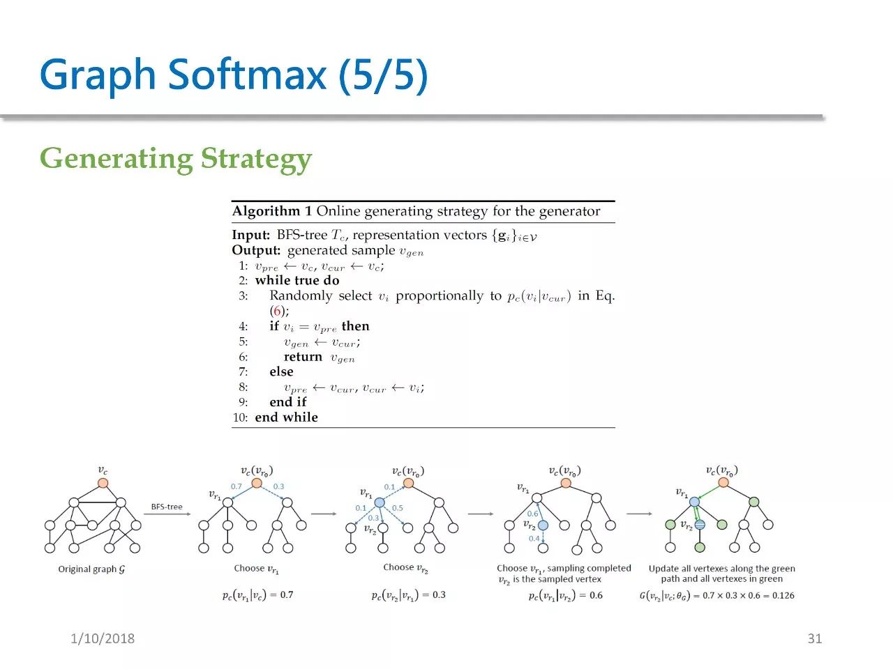
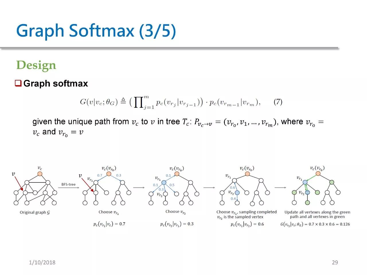
We have also designed a generation strategy. This generation strategy does not require calculating all probabilities before sampling; instead, it can compute and sample simultaneously.

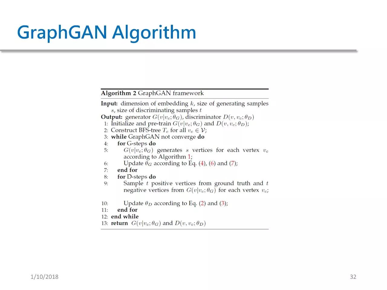
The algorithm for GraphGAN is as follows; the input is some hyperparameters, and we want to output the generative model G and the discriminative model D. Lines 3-12 show the iterative process of the algorithm. In each iteration, we repeat generating s points with the generator and use these points to update the parameters of θG.

Then, we repeatedly construct positive and negative samples to train D, which is done for stability reasons. We know that the stability of GAN training is an important issue.

Experiments

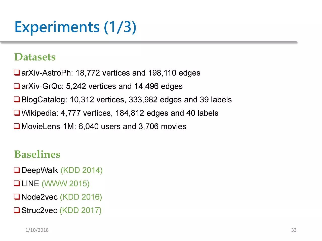
Our experimental datasets include five in total. The baseline methods selected are DeepWalk, LINE, Node2vec, and Struc2vec.

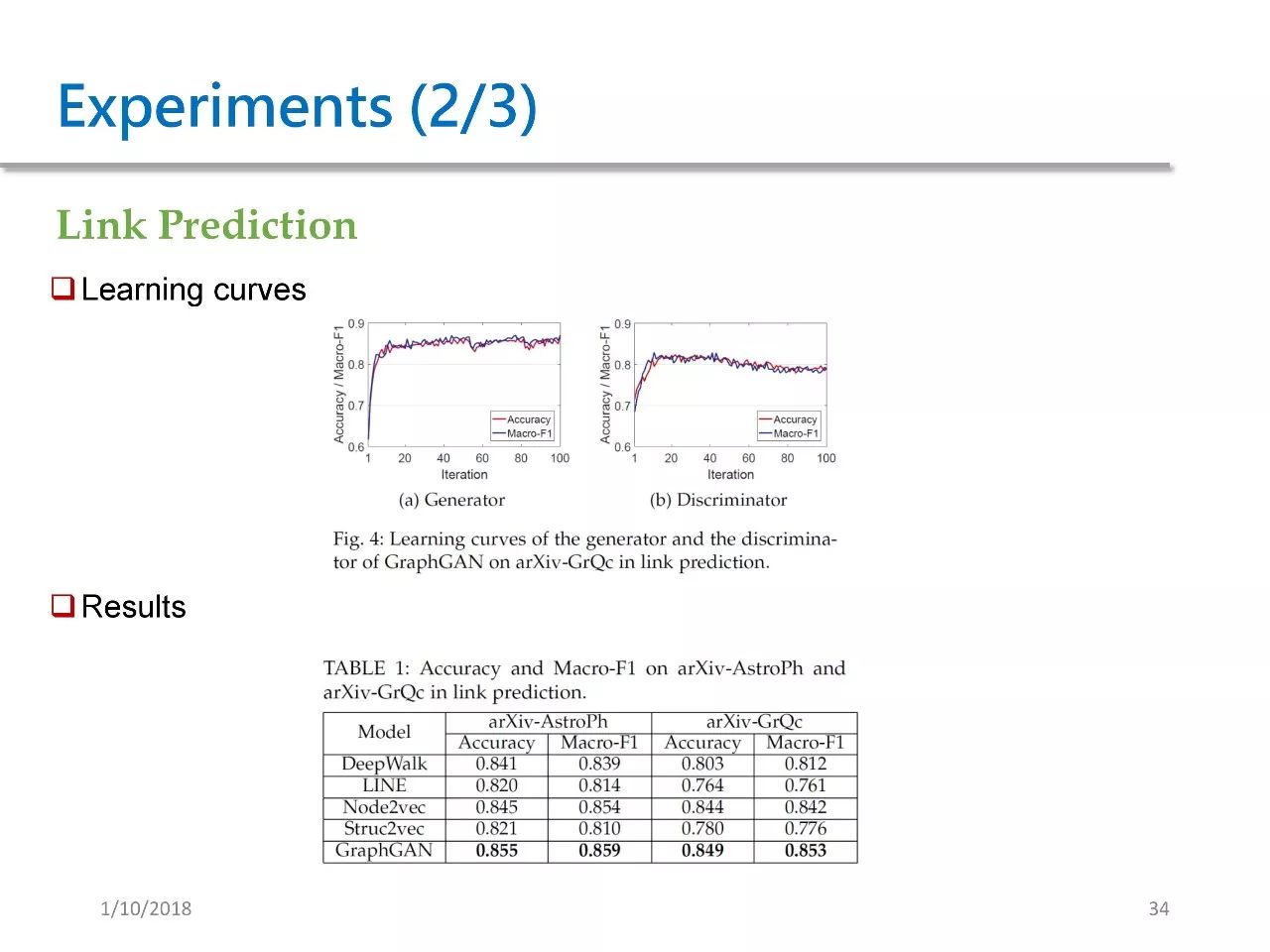
We applied GraphGAN in the following three testing scenarios. The first is link prediction, predicting the probability of an edge existing between two points. Figure 4 shows the learning curve of GraphGAN for the generator, which stabilizes quickly after about ten training rounds and maintains performance thereafter.

For D, its performance rises first, then shows a slow decline, which aligns with the GAN framework we described earlier. Table 1 shows that GraphGAN achieved the best results on both datasets.

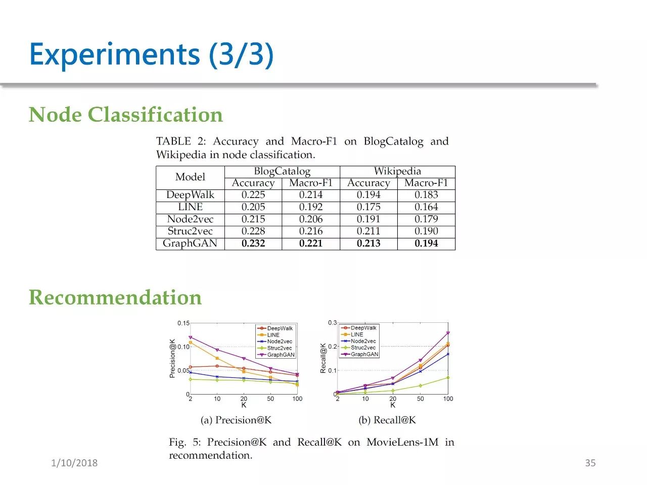
The second testing scenario is Node Classification, where we aim to classify nodes using the BlogCatalog and Wikipedia datasets. In such datasets, our method achieved the best results.

The third testing scenario is recommendation, using the MovieLens dataset, where our method also achieved the best results.

Conclusion

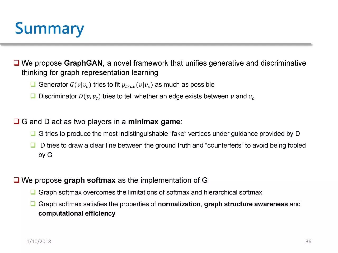
The GraphGAN proposed in this article is a framework that combines generative and discriminative models, where the generator fits Ptrue, and the discriminator attempts to determine whether there is an edge between two points.

G and D are essentially engaged in a minimax game, where G tries to produce fake points that cannot be distinguished by D, while D attempts to separate the real values from the fake points to avoid being deceived by G.

Additionally, we proposed a Graph Softmax as the implementation of G, overcoming the shortcomings of softmax and hierarchical softmax and possessing three good properties.

Other Applications of GRL

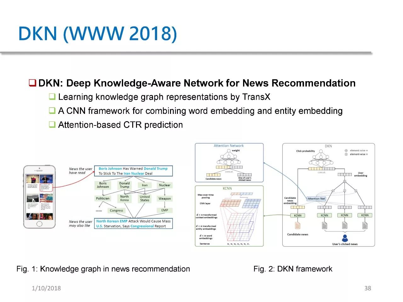
DKN is a paper we published at WWW 2018, which proposes a deep knowledge-aware network for news recommendation. In DKN, we combine entity embeddings and word embeddings from KG within a CNN framework, and propose an attention-based click-through rate prediction model.

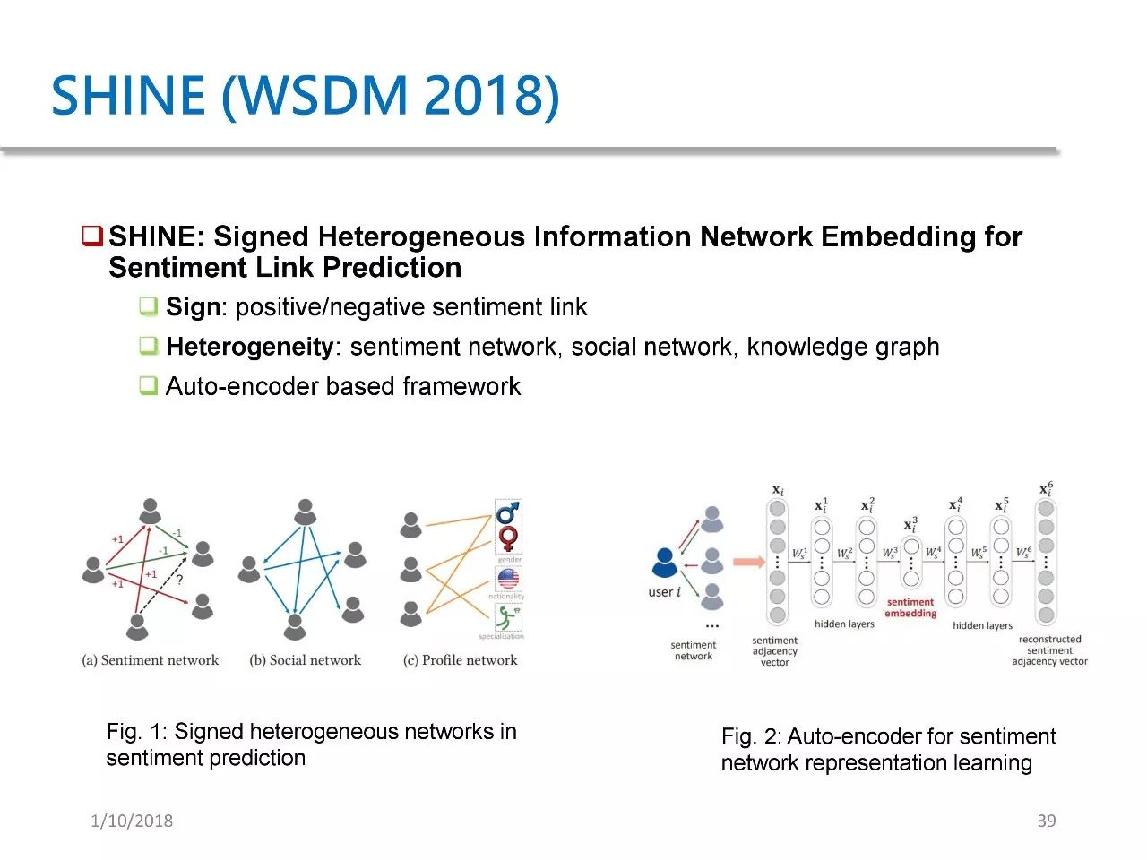
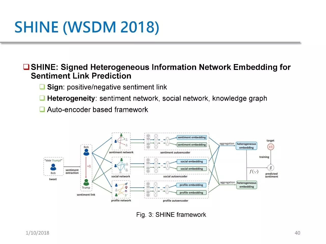
The second application is SHINE, a paper published at WSDM 2018. Its purpose is to predict the sentiment of Weibo users towards celebrities. We proposed a framework based on autoencoders, which is similar to SDNE, applied to three aspects and combined for sentiment prediction.

>>>> Get the complete PPT and video transcript

Follow the PaperWeekly WeChat official account and reply with 20180110 to get the download link.

Click the following titles to view past transcripts:

• Event Stream Research Based on Generative Models + NIPS 2017 Paper Interpretation

• Amazon Senior Applied Scientist Xiong Yuanjun: Progress in Behavior Understanding Research

• Tsinghua University Feng Jun: Relation Extraction and Text Classification Based on Reinforcement Learning

• Cross-Language Hierarchical Classification System Matching Based on Bilingual Topic Models

• Southeast University Gao Huan: Knowledge Graph Representation Learning

• GAN Model with Multi-Class Discriminator

About PaperWeekly

PaperWeekly is an academic platform for recommending, interpreting, discussing, and reporting cutting-edge research results in artificial intelligence. If you research or work in the AI field, feel free to click「Group Chat」 in the WeChat official account backend, and the assistant will bring you into the PaperWeekly group chat.