In 2014, the Visual Geometry Group at the University of Oxford and Google DeepMind developed a new convolutional neural network called VGGNet. VGGNet is a deeper deep convolutional neural network than AlexNet, and this model achieved second place in the 2014 ILSVRC competition, with GoogLeNet taking first place (which we will introduce later).
Paper: Very Deep Convolutional Networks for Large-Scale Image Recognition
1. Network Structure
The structure of VGG is similar to that of AlexNet, with the distinction that it is deeper but simpler in form. VGG consists of 5 convolutional layers, 3 fully connected layers, and 1 softmax output layer, separated by maxpooling layers. All hidden layer activation units use the ReLU function. In the original paper, the authors designed six network structures: A, A-LRN, B, C, D, and E, based on the number of sub-layers in the convolutional layers.
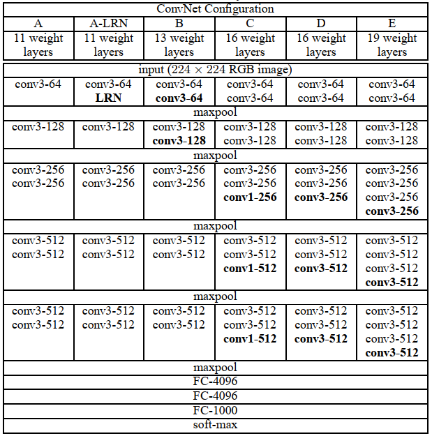
These six network structures are similar, each consisting of 5 convolutional layers and 3 fully connected layers, differing in the number of sub-layers in each convolutional layer, increasing sequentially from A to E, with total network depths ranging from 11 to 19 layers. The parameters of the convolutional layers are represented as “conv (receptive field size) – number of channels”; for example, conv3-64 indicates a 3×3 convolution kernel with 64 channels; max pooling is represented as maxpool, separating layers with maxpool; fully connected layers are represented as “FC – number of neurons”; for example, FC-4096 indicates a fully connected layer containing 4096 neurons; finally, there is the softmax layer.
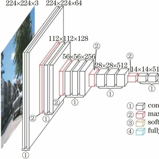
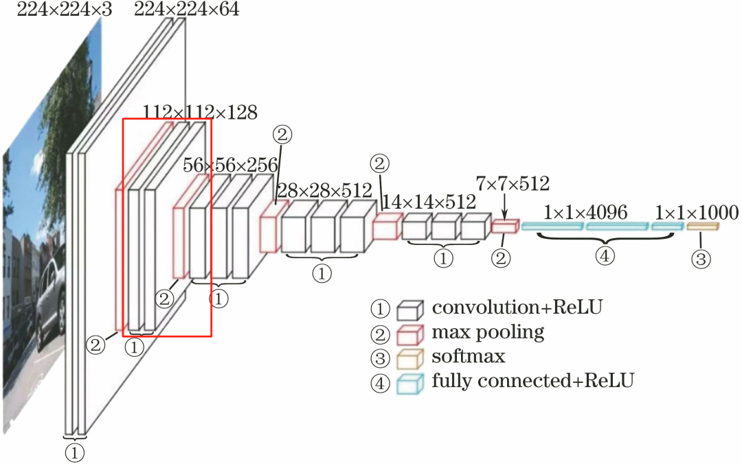
Among them, D represents the famous VGG16, and E represents the famous VGG19. Below, we will analyze the network structure of VGG in detail using VGG16 as an example. The structure of VGG16 is shown in the figure below:
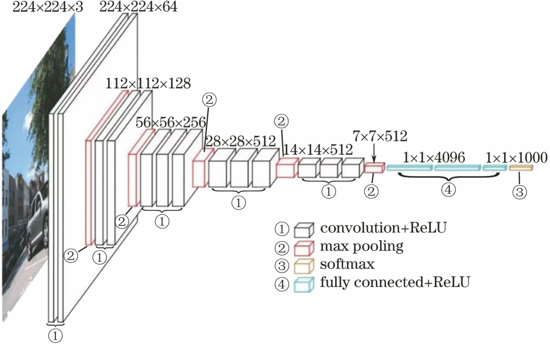
VGG16 contains a total of 16 sub-layers. The first convolutional layer consists of 2 conv3-64 layers, the second convolutional layer consists of 2 conv3-128 layers, the third convolutional layer consists of 3 conv3-256 layers, the fourth convolutional layer consists of 3 conv3-512 layers, and the fifth convolutional layer consists of 3 conv3-512 layers, followed by 2 FC4096 layers and 1 FC1000 layer. In total, there are 16 layers, which is the origin of the name VGG16.
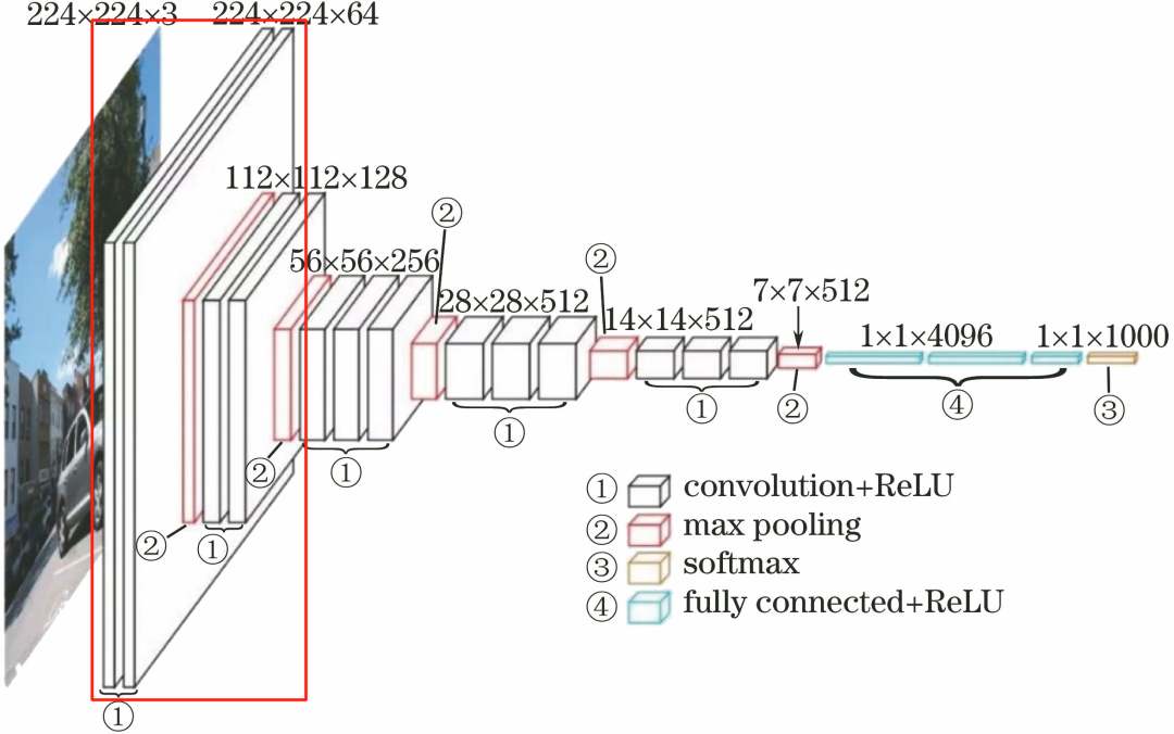
1.1 Input Layer
The input image size for VGG is 224x224x3.
1.2 First Convolutional Layer
The first convolutional layer consists of 2 conv3-64 layers.
The processing flow of this layer is: Convolution–>ReLU–> Convolution–>ReLU–>Pooling.
Convolution: The input is 224x224x3, using 64 3x3x3 convolution kernels for convolution, padding=1, stride=1. According to the formula:
(input_size + 2 * padding – kernel_size) / stride + 1=(224+2*1-3)/1+1=224
The output is 224x224x64.
ReLU: The feature map output from the convolutional layer is input into the ReLU function.
Convolution: The input is 224x224x64, using 64 3x3x64 convolution kernels for convolution, padding=1, stride=1. According to the formula:
(input_size + 2 * padding – kernel_size) / stride + 1=(224+2*1-3)/1+1=224
The output is 224x224x64.
ReLU: The feature map output from the convolutional layer is input into the ReLU function.
Pooling: Using 2×2 pooling units with stride=2 for max pooling operation. According to the formula:
(224+2*0-2)/2+1=112
The output for each group is 112x112x64.
1.3 Second Convolutional Layer
The second convolutional layer consists of 2 conv3-128 layers.
The processing flow of this layer is: Convolution–>ReLU–> Convolution–>ReLU–>Pooling.
Convolution: The input is 112x112x64, using 128 3x3x64 convolution kernels for convolution, padding=1, stride=1. According to the formula:
(input_size + 2 * padding – kernel_size) / stride + 1=(112+2*1-3)/1+1=112
The output is 112x112x128.
ReLU: The feature map output from the convolutional layer is input into the ReLU function.
Convolution: The input is 112x112x128, using 128 3x3x128 convolution kernels for convolution, padding=1, stride=1. According to the formula:
(input_size + 2 * padding – kernel_size) / stride + 1=(112+2*1-3)/1+1=112
The output is 112x112x128.
ReLU: The feature map output from the convolutional layer is input into the ReLU function.
Pooling: Using 2×2 pooling units with stride=2 for max pooling operation. According to the formula:
(112+2*0-2)/2+1=56
The output for each group is 56x56x128.
1.4 Third Convolutional Layer

The third convolutional layer consists of 3 conv3-256 layers.
The processing flow of this layer is: Convolution–>ReLU–> Convolution–>ReLU–>Pooling.
Convolution: The input is 56x56x128, using 256 3x3x128 convolution kernels for convolution, padding=1, stride=1. According to the formula:
(input_size + 2 * padding – kernel_size) / stride + 1=(56+2*1-3)/1+1=56
The output is 56x56x256.
ReLU: The feature map output from the convolutional layer is input into the ReLU function.
Convolution: The input is 56x56x256, using 256 3x3x256 convolution kernels for convolution, padding=1, stride=1. According to the formula:
(input_size + 2 * padding – kernel_size) / stride + 1=(56+2*1-3)/1+1=56
The output is 56x56x256.
ReLU: The feature map output from the convolutional layer is input into the ReLU function.
Pooling: Using 2×2 pooling units with stride=2 for max pooling operation. According to the formula:
(56+2*0-2)/2+1=28
The output for each group is 28x28x256.
1.5 Fourth Convolutional Layer

The fourth convolutional layer consists of 3 conv3-512 layers.
The processing flow of this layer is: Convolution–>ReLU–> Convolution–>ReLU–>Pooling.
Convolution: The input is 28x28x256, using 512 3x3x256 convolution kernels for convolution, padding=1, stride=1. According to the formula:
(input_size + 2 * padding – kernel_size) / stride + 1=(28+2*1-3)/1+1=28
The output is 28x28x512.
ReLU: The feature map output from the convolutional layer is input into the ReLU function.
Convolution: The input is 28x28x512, using 512 3x3x512 convolution kernels for convolution, padding=1, stride=1. According to the formula:
(input_size + 2 * padding – kernel_size) / stride + 1=(28+2*1-3)/1+1=28
The output is 28x28x512.
ReLU: The feature map output from the convolutional layer is input into the ReLU function.
Pooling: Using 2×2 pooling units with stride=2 for max pooling operation. According to the formula:
(28+2*0-2)/2+1=14
The output for each group is 14x14x512.
1.6 Fifth Convolutional Layer
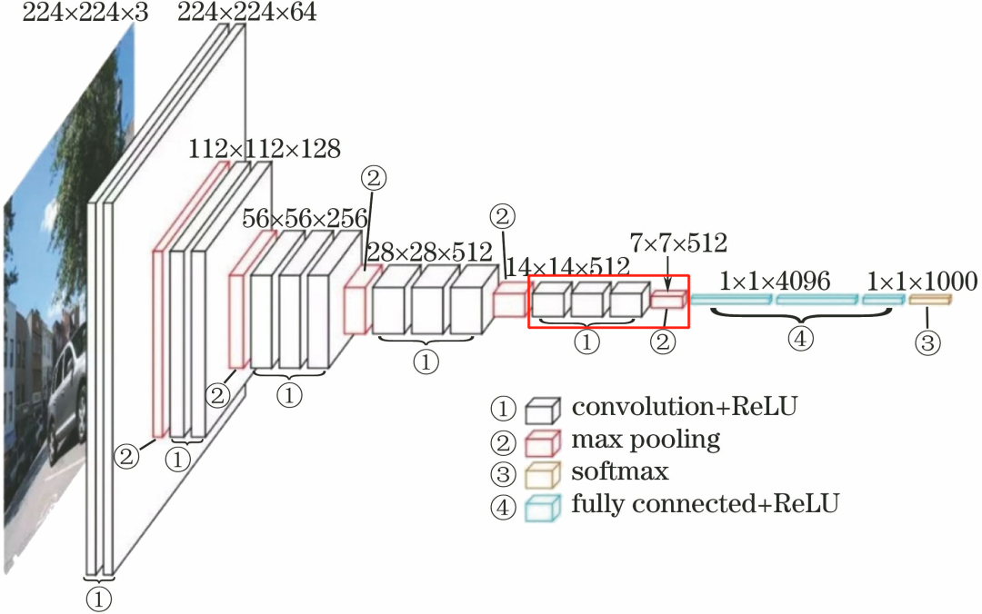
The fifth convolutional layer consists of 3 conv3-512 layers.
The processing flow of this layer is: Convolution–>ReLU–> Convolution–>ReLU–>Pooling.
Convolution: The input is 14x14x512, using 512 3x3x512 convolution kernels for convolution, padding=1, stride=1. According to the formula:
(input_size + 2 * padding – kernel_size) / stride + 1=(14+2*1-3)/1+1=14
The output is 14x14x512.
ReLU: The feature map output from the convolutional layer is input into the ReLU function.
Pooling: Using 2×2 pooling units with stride=2 for max pooling operation. According to the formula:
(14+2*0-2)/2+1=7
The output for each group is 7x7x512.
1.7 First Fully Connected Layer
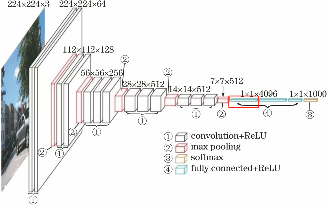
The first fully connected layer FC4096 consists of 4096 neurons.
The processing flow of this layer is: FC–>ReLU–>Dropout.
FC: The input is 7x7x512 feature map, unfolded into a one-dimensional vector of 7*7*512, i.e., 7*7*512 neurons, with an output of 4096 neurons.
ReLU: The computation results of these 4096 neurons go through the ReLU activation function.
Dropout: Randomly disconnect connections of some neurons in the fully connected layer to prevent overfitting by deactivating certain neurons.
1.8 Second Fully Connected Layer

The second fully connected layer FC4096 consists of 4096 neurons.
The processing flow of this layer is: FC–>ReLU–>Dropout.
FC: The input is 4096 neurons, with an output of 4096 neurons.
ReLU: The computation results of these 4096 neurons go through the ReLU activation function.
Dropout: Randomly disconnect connections of some neurons in the fully connected layer to prevent overfitting by deactivating certain neurons.
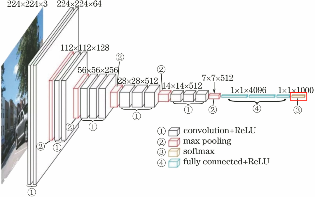
1.9 Third Fully Connected Layer

The third fully connected layer FC1000 consists of 1000 neurons, corresponding to the 1000 categories of the ImageNet dataset.
The processing flow of this layer is: FC.
FC: The input is 4096 neurons, with an output of 1000 neurons.
1.10 Softmax Layer
The flow of this layer is: Softmax
Softmax: The computation results of these 1000 neurons go through the Softmax function, outputting the predicted probability values corresponding to the 1000 categories.
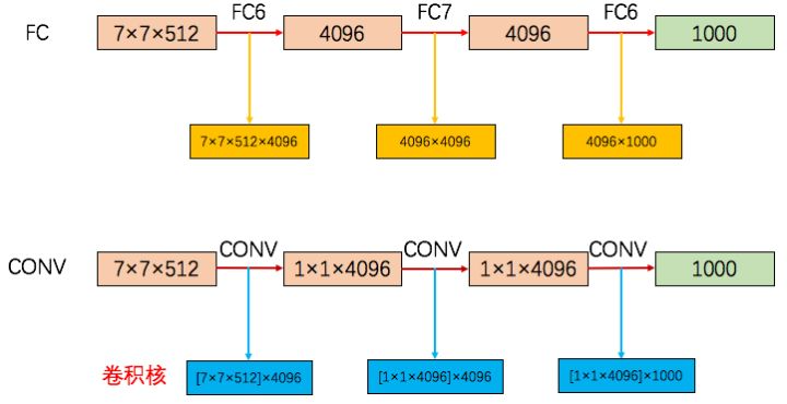
2. Fully Convolutional Network
Next, we will introduce the content of sections 1.7, 1.8, and 1.9. These three sections discuss fully connected networks; VGG16 uses fully connected networks during training. However, during the testing and validation phase, the network structure is slightly different, as the authors replace all fully connected layers with convolutional networks.
First, let’s introduce the approach!
2.1 First Fully Connected Layer
The input is 7x7x512 feature map, using 4096 7x7x512 convolution kernels for convolution. Since the kernel size matches the input size, each coefficient in the kernel corresponds to a pixel value in the input. According to the formula:
(input_size + 2 * padding – kernel_size) / stride + 1=(7+2*0-7)/1+1=1
The output is 1x1x4096. This is equivalent to 4096 neurons, but it belongs to the convolutional layer.
2.2 Second Fully Connected Layer
The input is 1x1x4096 feature map, using 4096 1x1x4096 convolution kernels for convolution. Since the kernel size matches the input size, each coefficient in the kernel corresponds to a pixel value in the input. According to the formula:
(input_size + 2 * padding – kernel_size) / stride + 1=(1+2*0-1)/1+1=1
The output is 1x1x4096. This is equivalent to 4096 neurons, belonging to the convolutional layer.
2.3 Third Fully Connected Layer
The input is 1x1x4096 feature map, using 1000 1x1x4096 convolution kernels for convolution. Since the kernel size matches the input size, each coefficient in the kernel corresponds to a pixel value in the input. According to the formula:
(input_size + 2 * padding – kernel_size) / stride + 1=(1+2*0-1)/1+1=1
The output is 1x1x1000. This is equivalent to 1000 neurons, belonging to the convolutional layer.
After obtaining the 1x1x1000 output, it is finally passed through the softmax layer for class prediction.
2.4 Why Convert Fully Connected Layers to Fully Convolutional Layers?
The authors converted the three fully connected layers into 1 7×7 and 2 1×1 convolutional layers. As seen in the figure below, taking the first fully connected layer as an example, the input to FC6 is 7×7×512, and the output is 4096 (which can also be seen as 1×1×4096). Therefore, to convert to a convolutional layer, the input needs to be reduced in size (from 7×7 to 1×1) and increased in depth (from 512 to 4096). To reduce the 7×7 to 1×1, a convolution kernel of size 7×7 is used, with the number of kernels set to 4096, i.e., the convolution kernel is 7×7×4096 (the notation [7×7×512]×4096 in the figure indicates that there are 4096 such [7×7×512] convolution kernels, and 7×7×4096 is a simplified form that ignores the input depth).
Why convert fully connected layers to fully convolutional layers during model testing? The most direct reason is to allow the network model to accept arbitrary input sizes.
When we introduced it earlier, we limited the input image size to 224x224x3. If the next three layers are all fully connected, any image larger than 224 will need to be cropped, resized, or otherwise processed to unify the image size to 224x224x3 to meet the input requirements of the subsequent fully connected layers. However, we cannot guarantee that each crop will retain the key targets in the image; cropping may remove critical information, impacting the model’s testing accuracy.
(The output is a classification score map, where the number of channels equals the number of categories, and the spatial resolution depends on the input image size. In the end, to obtain a fixed-size classification score vector, the score map is spatially averaged (summed – pooled). We also use horizontal flipping to augment the test set; the average of the softmax classification probabilities on the original and flipped images serves as the final score for the image.)
Using fully convolutional layers, even if the image size exceeds 224x224x3, the final score map obtained after passing through the softmax layer is not 1x1x1000; for example, it could be 2x2x1000, where the 1000 channels correspond to the number of categories, and the spatial resolution of 2×2 depends on the input image size. The score map is then spatially averaged (summed pooling), resulting in a 1x1x1000. Finally, the scores of the 1000 channels are compared, and the larger value is taken as the predicted category.
The advantage of this approach is that it greatly reduces the impact of feature location on classification.
To illustrate:
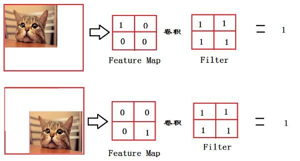
From the above image, we can see that the cat is in different positions in the original image; if we use fully connected layers, it is easy for the cropped image to lose key targets. However, using fully convolutional layers allows direct convolution on the original image, and the final score map, after pooling, yields a score of 1, regardless of where the cat is in the image, ensuring correct classification. By preserving the original image and using fully convolutional layers, it means that we don’t care where the cat is; we just want to find the cat, allowing the model to identify the presence of the cat by integrating the feature map into a single value. If this value is large, it indicates the presence of a cat; if small, it likely indicates its absence! The relationship with the cat’s position in the image becomes less significant, greatly enhancing robustness.
3. Characteristics of VGG Network
3.1 Simple Structure
Although VGG has many layers, with total network depths ranging from 11 to 19 layers, its overall structure is still relatively simple. In summary, VGG consists of 5 convolutional layers (with different numbers of sub-layers for each), 3 fully connected layers, and a softmax output layer, separated by maxpooling layers, with all hidden layer activation units using the ReLU function.
3.2 Small Convolution Kernels
Small convolution kernels are an important feature of VGG. VGG does not use larger convolution kernel sizes (such as 7×7) as in AlexNet but achieves similar performance by reducing the kernel size (3×3) and increasing the number of convolution sub-layers (VGG: from 1 to 4 convolution sub-layers, AlexNet: 1 sub-layer).
VGG uses multiple smaller convolution kernels (3×3) in place of a single larger convolution kernel; the authors believe that stacking two 3×3 convolutions achieves the same receptive field size as a single 5×5 convolution, and stacking three 3×3 convolutions achieves the same receptive field as a 7×7 convolution. The schematic diagram is shown below:
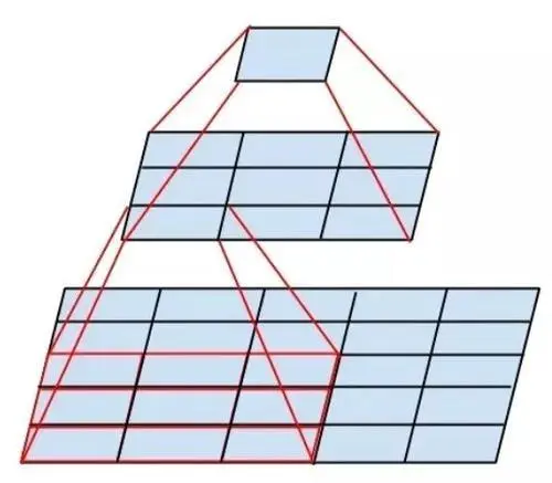
The benefits of using 3×3 small convolution kernels are twofold:
First, it significantly reduces the number of model parameters. For example, using two 3×3 convolution kernels instead of one 5×5 kernel, with C channels, the parameter count for one 5×5 kernel is 5*5*C, while for two 3×3 kernels, the parameter count is 2*3*3*C, reducing parameters by 28%. Additionally, using small convolution kernels with smaller strides can prevent loss of detail information.
Second, multiple convolution layers (with non-linear activation functions after each convolution layer) increase non-linearity, enhancing model performance.
Furthermore, we note that in the VGG structure D, 1×1 convolution kernels are also used, which can increase model non-linearity (with subsequent non-linear activation functions) without changing the receptive field. They can also be used to integrate information across channels and output a specified number of channels. Reducing the number of channels means dimensionality reduction, while increasing the number of channels means dimensionality expansion.
3.3 Smaller Pooling Kernels
Compared to AlexNet’s 3×3 pooling kernel, VGG uses only 2×2 pooling kernels.
3.4 More Channels, Broader Features
Each channel represents a feature map, and more channels indicate richer image features. The number of channels in the first layer of VGG is 64, and this doubles in each subsequent layer, reaching a maximum of 512 channels. The increase in the number of channels allows for more information to be extracted.
3.5 Deeper Layers
By using consecutive 3×3 small convolution kernels instead of larger kernels, the network depth increases, and padding ensures that the image size does not decrease during convolution. Only small 2×2 pooling units are used to reduce the image size.
3.6 Fully Connected to Convolution
This section has already been introduced in the fully convolutional network.
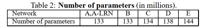
3.7 Model Parameters
Although the depth of the six network structures A, A-LRN, B, C, D, and E increases from 11 to 19 layers, the number of parameters does not change significantly because they mostly use small convolution kernels, with parameters primarily concentrated in the fully connected layers.
3.8 Others
The A-LRN network structure uses LRN layers (local response normalization), which were also used in the AlexNet network. However, the authors found that LRN did not improve performance, so it did not appear in the other network structures.
From 11 layers in A to 19 layers in E, the increase in network depth significantly reduces the top-1 and top-5 error rates.
The authors of VGG compared the B network to a shallower network that used one 5×5 convolution kernel instead of B’s two 3×3 kernels, and the results showed that multiple small convolution kernels perform better than a single large convolution kernel.
For more details and experimental comparison results regarding VGG, we recommend reading the original paper directly!
Handwritten CNN Series:
Handwritten CNN Classic Network LeNet-5 (Theoretical Part)
Handwritten CNN Classic Network LeNet-5 (MNIST Practical Part)
Handwritten CNN Classic Network LeNet-5 (CIFAR10 Practical Part)
Handwritten CNN Classic Network LeNet-5 (Custom Practical Part)
Handwritten CNN Classic Network AlexNet (Theoretical Part)
Handwritten CNN Classic Network AlexNet (PyTorch Practical Part)
If you find this article useful, please like or share it with your friends!
Recommended Reading
(Click the title to jump to read)
Useful | Selected Historical Articles from Official Account
My Deep Learning Entry Route
My Machine Learning Entry Roadmap
Important!
The annual technical article electronic version PDF from AI Youdao is here!
Scan the QR code below to add AI Youdao assistant WeChat, you can apply to join the group and obtain the complete technical article collection PDF for 2020 (please note:Join + Location + School/Company. For example:Join + Shanghai + Fudan.)

Long press to scan the code and apply to join the group
(Due to a large number of applicants, please be patient)