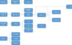
Comprehensive Summary of Optimization Algorithms in Machine Learning

Introduction

For almost all machine learning algorithms, whether supervised learning, unsupervised learning, or reinforcement learning, they ultimately boil down to solving optimization problems. Therefore, optimization methods play a central role in the derivation and implementation of machine learning algorithms. In this article, I will provide a comprehensive summary of the optimization algorithms used in machine learning, clarifying their direct relationships to help you understand this part of knowledge from a global perspective.

Mathematical Models Required by Machine Learning

Almost all machine learning algorithms ultimately reduce to finding the extreme value of an objective function, that is, an optimization problem. For example, in supervised learning, we want to find the best mapping function f(x) that minimizes the loss function for training samples (minimizing empirical risk or structural risk):

Comprehensive Summary of Optimization Algorithms in Machine Learning

Here, N is the number of training samples, L is the loss function for a single sample, w is the model parameters to be solved, which are the parameters of the mapping function, xi is the feature vector of the sample, and yi is the label value of the sample.

Alternatively, we can find an optimal probability density function p(x) that maximizes the log-likelihood function for training samples (maximum likelihood estimation):

Here, θ is the model parameters to be solved, which are the parameters of the probability density function.

For unsupervised learning, taking clustering algorithms as an example, the algorithm aims to minimize the sum of distances of each class’s samples to the class center:

Here, k is the number of types, x is the sample vector, μi is the class center vector, and Si is the sample set of the i-th class.

For reinforcement learning, we want to find an optimal policy, that is, the mapping function from state s to action a (deterministic policy; for a non-deterministic policy, it is the probability of executing each action):

To maximize the cumulative reward obtained after executing the action a determined by this policy function given any state:

Here, the state value function is used.

Overall, the core goal of machine learning is to provide a model (generally a mapping function) and then define an evaluation function (objective function) for the quality of this model, solving for the maximum or minimum of the objective function to determine the model parameters, thus obtaining the desired model. In these three key steps, the first two are the problems that machine learning studies, establishing mathematical models. The third problem is a pure mathematical problem, namely optimization methods, which is the core of this article.

Classification of Optimization Algorithms

For optimization objective functions of machine learning algorithms with various forms and characteristics, we have found various solution algorithms suitable for them. Except for a few problems that can be solved optimally by brute force search, we divide the optimization algorithms used in machine learning into two types (this article does not consider stochastic optimization algorithms such as simulated annealing, genetic algorithms, etc.):

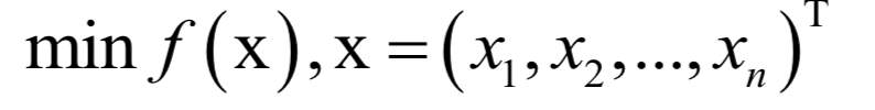
Analytical Solution
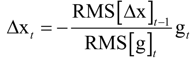
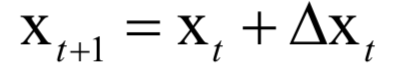
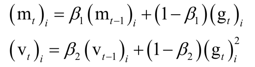
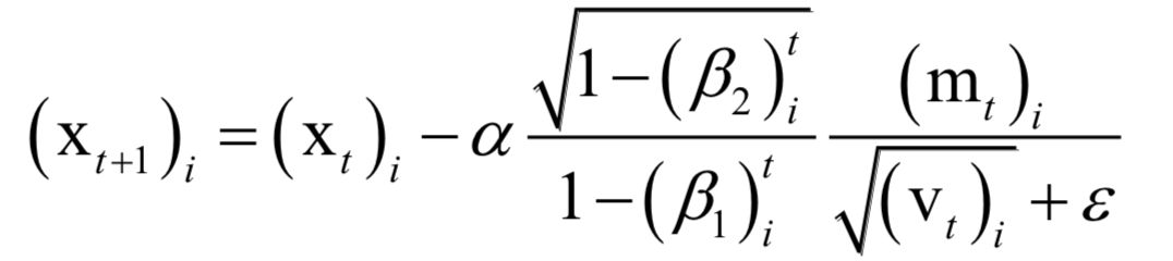
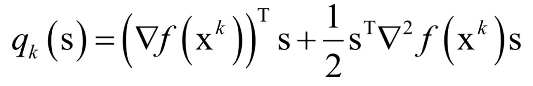
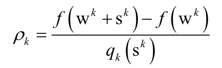
Numerical Optimization

The former provides an exact analytical solution to an optimization problem, generally a theoretical result. The latter is used when it is very difficult to give an exact calculation formula for the extreme point, using numerical methods to approximate the optimal point. In addition, there are other solution ideas such as divide and conquer, dynamic programming, etc. We will list them separately later. A good optimization algorithm needs to meet:

Can correctly find extreme points in various situations
Fast speed

The following figure shows the classification of these algorithms and their relationships:

Next, we will elaborate according to this diagram.

Fermat’s Theorem

For a differentiable function, the unified approach to finding its extreme value is to find the points where the derivative is zero, that is, Fermat’s theorem. This theorem in calculus states that for a differentiable function, the derivative must be zero at the extreme points:

For multivariable functions, the gradient must be zero:

Points where the derivative is zero are called stationary points. It is important to note that having a derivative of zero is only a necessary condition for a function to attain an extreme value, not a sufficient condition; it is merely a suspected extreme point. Whether it is an extreme value, whether it is a maximum or minimum, also requires checking higher-order derivatives. For univariate functions, assuming x is a stationary point:

If f”(x) > 0, then it is a minimum at that point
If f”(x) < 0, then it is a maximum at that point
If f”(x) >= 0, further higher-order derivatives need to be checked

For multivariable functions, assuming x is a stationary point:

If the Hessian matrix is positive definite, the function has a minimum at that point
If the Hessian matrix is negative definite, the function has a maximum at that point
If the Hessian matrix is indefinite, further checks are needed (this part is incorrect)

At points where the derivative is zero, the function may not attain an extreme value, which is called a saddle point. The following diagram is an example of a saddle point (from SIGAI Cloud Laboratory):

In addition to saddle points, optimization algorithms may also encounter another problem: the local extreme value problem, where a stationary point is an extreme point but not a global extreme point. If we impose constraints on the optimization problem, we can effectively avoid these two issues. A typical example is convex optimization, which requires that the feasible region of the optimization variables is a convex set and the objective function is a convex function.

Although stationary points are only a necessary condition for a function to attain an extreme value and not a sufficient condition, if we have found stationary points, it is much easier to judge and filter whether they are extreme points. Whether theoretical results or numerical optimization algorithms, they generally aim to find stationary points as the goal of finding extreme points. For univariate functions, we first find the derivative, then solve the equation where the derivative equals zero to find all stationary points. For multivariable functions, we take partial derivatives with respect to each variable, set them to zero, and solve the system of equations to achieve all stationary points. These are the basic methods taught in calculus. Fortunately, in machine learning, many objective functions are differentiable, so we can use this method.

Lagrange Multiplier Method

Fermat’s theorem gives the necessary conditions for the extreme value of a function without constraints. For some practical application problems, there are generally equality or inequality constraints. For extreme value problems with equality constraints, the classic solution is the Lagrange multiplier method.

For the following problem:

Construct the Lagrange multiplier function:

At the optimal point, the derivatives with respect to x and the multiplier variables λi must both equal zero:

Solving this equation gives the optimal solution. For a more detailed explanation of the Lagrange multiplier method, you can read any advanced mathematics textbook. The places where the Lagrange multiplier method is used in machine learning include:

Principal Component Analysis
Linear Discriminant Analysis
Laplacian Eigenmaps in Manifold Learning
Hidden Markov Model

KKT Conditions

KKT conditions are a generalization of the Lagrange multiplier method, used to solve functions with both equality and inequality constraints. For the following optimization problem:

Similar to the Lagrange duality approach, the KKT conditions construct the following multiplier function:

λ and μ are called KKT multipliers. At the optimal solution x*, the following conditions should be satisfied:

The equality constraint hj(x*)=0 and the inequality constraint gk(x*)<=0 are constraints that must be satisfied, ▽xL(x*)=0, which is the same as the previous Lagrange multiplier method. The only additional condition is regarding gi(x):

KKT conditions are only necessary conditions for attaining extreme values and not sufficient conditions. In machine learning, KKT conditions are used in places such as:

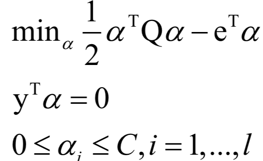
Support Vector Machine (SVM)

Numerical Optimization Algorithms

The three methods discussed earlier can be used in theoretical derivations and in cases where certain equations can obtain root-finding formulas (such as linear functions, maximum likelihood estimation of normal distributions), but for the vast majority of functions, the equations where the gradient equals zero cannot be directly solved, such as equations containing transcendental functions like exponential functions and logarithmic functions. For these unsolvable equations, we can only use approximate algorithms for solving, namely numerical optimization algorithms. These numerical optimization algorithms generally utilize the derivative information of the objective function, such as first-order derivatives and second-order derivatives. If first-order derivatives are used, they are called first-order optimization algorithms. If second-order derivatives are used, they are called second-order optimization algorithms.

In engineering implementation, iterative methods are usually adopted, starting from an initial point x0, repeatedly moving from xk to the next point xk+1 using some rules, constructing such a sequence until it converges to the point where the gradient equals zero. That is, the following limit holds:

These rules generally utilize first-order derivative information, namely the gradient; or second-order derivative information, namely the Hessian matrix. Thus, the core of the iterative method is to obtain an iteration formula that determines the next point based on the previous point:

Gradient Descent Method

The gradient descent method searches in the opposite direction of the gradient, utilizing the first-order derivative information of the function. The iterative formula of the gradient descent method is:

According to the first-order Taylor expansion of the function, in the negative gradient direction, the function value decreases. As long as the learning rate is set small enough and does not reach the point where the gradient equals zero, the function value will definitely decrease at each iteration. The reason for setting the learning rate to a very small positive number is to ensure that the updated xk+1 is within the neighborhood of the previous value xk, thereby ignoring the higher-order terms in the Taylor expansion and ensuring that the function value decreases during iterations.

The gradient descent method and its variants are widely used in machine learning, especially in deep learning. )

Momentum Term

To speed up the convergence of the gradient descent method and reduce oscillation, a momentum term is introduced. The momentum term accumulates the gradient values from previous iterations, and the parameter update formula after adding this term is:

Where Vt+1 is the momentum term, which replaces the previous gradient term. The calculation formula for the momentum term is:

It is a weighted average of the previous momentum term and the current gradient value, where α is the learning rate and μ is the momentum term coefficient. If expanded according to time t, then at the t-th iteration, all gradient values from the 1st to the t-th iteration are used, and the old gradient values decay exponentially with a coefficient of μt:

The momentum term accumulates the gradient values from previous iterations, allowing the current iteration to move forward in the direction of previous inertia.

AdaGrad Algorithm

AdaGrad is the most direct improvement of the gradient descent method. The gradient descent method relies on a manually set learning rate, which can be difficult to set appropriately. If set too small, convergence is too slow; if set too large, it may lead to non-convergence of the algorithm.

AdaGrad dynamically adjusts the learning rate based on the historical gradient values from previous iterations, and each component of the optimization variable vector X has its own learning rate. The parameter update formula is:

Where α is the learning factor, gt is the gradient vector of the parameters at the t-th iteration, and ε is a very small positive number to avoid division by zero. The subscript i denotes the component of the vector. The only difference from standard gradient descent is the additional term in the denominator, which accumulates the historical gradient values up to this iteration to generate the coefficient for gradient descent. According to this formula, the larger the absolute value of the historical derivatives, the smaller the component learning rate, and vice versa. Although it achieves an adaptive learning rate, this algorithm still has problems: it requires manually setting a global learning rate α, and as time accumulates, the denominator in the formula will grow larger, causing the learning rate to approach zero, making it impossible to effectively update parameters.

RMSProp Algorithm

RMSProp is an improvement over AdaGrad, avoiding the problem of the learning rate approaching zero due to long-term accumulation of gradient values. The specific approach is to construct a vector RMS from the gradient values, initialized to zero, and accumulate the historical squared gradient values according to a decay coefficient. The update formula is:

AdaGrad directly accumulates all historical squared gradients, while here, the historical squared gradient values are accumulated after decaying with δt. The parameter update formula is:

Where δ is a manually set parameter, and like AdaGrad, it also requires a manually specified global learning rate α.

AdaDelta Algorithm

AdaDelta is also an improvement over AdaGrad, avoiding the problem of the learning rate approaching zero due to long-term accumulation of gradient values, and it also removes the dependency on manually set global learning rates. Assuming the parameter to be optimized is x, the gradient value calculated during the t-th iteration of the gradient descent method is gt. The algorithm first initializes the following two vectors to zero:

Where E[g2] is the cumulative value of the squared gradient (calculated separately for each component), and the update formula is:

Here, g2 is the square of each element of the vector, and all subsequent calculations are performed for each component of the vector. Next, calculate the following RMS quantity:

This is also a vector, calculated separately for each component of the vector. Then calculate the update value for the parameters:

The calculation formula for RMS[Δx]t-1 is similar to this. This update value is also constructed through the gradient, but the learning rate is determined by the historical gradient values. The update formula is:

The iterative formula for parameter updates is:

Adam Algorithm

The Adam algorithm integrates adaptive learning rates with momentum terms. The algorithm constructs two vectors m and v from the gradient, the former being the momentum term and the latter accumulating the squared gradients, used to construct adaptive learning rates. Their initial values are zero, and the update formula is:

Where β1 and β2 are manually specified parameters, and i is the index of the vector component. Relying on these two values constructs the update value for the parameters, and the parameter update formula is:

Here, m is similar to the momentum term, and v is used to construct the learning rate.

Stochastic Gradient Descent

Assuming the training sample set has N samples, the goal of supervised learning algorithms during training is to optimize the average loss function over this dataset:

Where L(w, xi, yi) is the loss function for a single training sample (xi, yi), w is the parameters to be learned, r(w) is the regularization term, and λ is the weight of the regularization term. When the number of training samples is large, if we use all samples for each iteration during training, the computational cost is too high. As an improvement, we can select a batch of samples during each iteration and define the loss function over these samples.

Batch stochastic gradient descent uses a random approximation of the objective function in each iteration, that is, only M < N randomly selected samples to approximate the loss function. The objective function to optimize in each iteration becomes:

Stochastic gradient descent converges in a probabilistic sense.

Newton’s Method

Newton’s method is a second-order optimization technique that utilizes first-order and second-order derivative information to directly find points where the gradient equals zero. The iterative formula of Newton’s method is:

Where H is the Hessian matrix, and g is the gradient vector. Newton’s method cannot guarantee that the function value decreases at each iteration, nor can it guarantee convergence to a minimum point. In implementation, a learning rate also needs to be set, for the same reason as the gradient descent method, which is to ignore higher-order terms in the Taylor expansion. The learning rate is usually set using line search techniques.

In implementation, we usually do not directly compute the inverse of the Hessian matrix but instead solve the following linear equation:

Its solution d is called the Newton direction. The termination criterion for the iteration is that the gradient value is sufficiently close to zero or the maximum specified number of iterations is reached.

Newton’s method has a faster convergence speed than the gradient descent method, but requires calculating the Hessian matrix at each iteration and solving a linear equation, which is computationally intensive. Additionally, if the Hessian matrix is non-invertible, this method fails.

Newton’s method has practical applications in logistic regression, AdaBoost algorithms, and other machine learning algorithms.

Quasi-Newton Method

Newton’s method requires calculating the Hessian matrix and solving a linear equation with that matrix as the coefficient matrix at each iteration, and the Hessian matrix may be non-invertible. To address this, some improved methods have been proposed, with the typical representative being the quasi-Newton method. The idea of the quasi-Newton method is to not compute the Hessian matrix of the objective function and then invert it, but to obtain an approximate inverse Hessian matrix through other means. The specific approach is to construct a positive definite symmetric matrix that approximates the Hessian matrix or its inverse, and use this matrix for Newton’s method iterations.

All these major numerical optimization algorithms can be freely experimented with on the SIGAI cloud laboratory:

www.sigai.cn

By constructing the objective function and specifying the parameters and initial values of the optimization algorithm, the algorithm’s running process can be visualized, and the results of solving with different parameters can be compared.

Trust Region Newton Method

The standard Newton method may not converge to an optimal solution, nor can it guarantee that the function value will decrease according to the iteration sequence. This problem can be solved by adjusting the step size of the Newton direction; currently, two common methods are line search and trust region methods. The trust region Newton method is a variant of the truncated Newton method used to solve optimization problems with bounded constraints. In each iteration of the trust region Newton method, there is an iteration sequence xk, a trust region size Δk, and a quadratic objective function:

This expression can be obtained through a Taylor expansion, ignoring terms of order higher than quadratic, which is the approximate decrease in function value:

The algorithm seeks a sk that approximately minimizes qk(S) under the constraint ||S|| <= Δk. It then checks the following ratio to update wk and Δk:

This is the ratio of the actual reduction in function value to the predicted reduction in function value caused by the quadratic approximation model. Based on previous calculations, the size of the trust region is dynamically adjusted.

The trust region Newton method has practical applications in logistic regression and the solution of linear support vectors; specific details can be read in the liblinear open-source library.

Divide and Conquer Method

The divide and conquer method is an algorithm design idea that breaks a large problem into sub-problems for solving. Based on the solutions to the sub-problems, the solution to the entire problem is constructed. In optimization methods, the specific approach is to adjust only a part of the optimization vector’s components during each iteration while keeping the other components fixed.

Coordinate Descent Method

The basic idea of the coordinate descent method is to optimize one variable at a time, which is a form of the divide and conquer method. Assuming the optimization problem to be solved is:

The process of solving the coordinate descent method is to select one component xi for optimization at each step while keeping the other components fixed, thus transforming a multivariable function’s extreme value problem into a univariate function’s extreme value problem. If the problem to be solved is large in scale, this approach can effectively speed up the process.

The coordinate descent method has practical applications in logistic regression and the solution of linear support vectors; specific details can be read in the liblinear open-source library.

SMO Algorithm

The SMO algorithm is also a form of the divide and conquer method used to solve the dual problem of support vector machines. The dual problem after adding slack variables and kernel functions is:

The core idea of the SMO algorithm is to optimize two components αi and αj from the optimization variables at a time, keeping the other components fixed, thereby ensuring that the equality constraint is satisfied. The reason for selecting two variables for optimization instead of one is that there is an equality constraint here; if only one variable’s value is adjusted, the equality constraint will be violated.

Assuming the selected two components are αi and αj, while keeping the other components fixed as constants, the objective function for these two variables is a bivariate quadratic function. This problem also has equality and inequality constraints. The closed-form solution for this subproblem can be directly obtained, which is the extreme value of a univariate quadratic function within a certain interval.

Stage-wise Optimization

The stage-wise optimization approach is to fix part of the optimization variable X during each iteration while optimizing another part of the variable b; then fix b and optimize a. This process is repeated until convergence to the optimal solution.

The AdaBoost algorithm is a typical representative of this method. The AdaBoost algorithm uses an exponential loss function during training:

Since the strong classifier is a weighted sum of multiple weak classifiers, substituting the above loss function gives the objective function to optimize during algorithm training:

Here, the exponential loss function is split into two parts: the existing strong classifier Fj−1 and the current weak classifier f’s loss function on the training samples. The former has already been obtained in previous iterations, so it can be treated as a constant. Thus, the objective function can be simplified to:

Where:

This problem can be solved in two steps: first, treat the weak classifier’s weight β as a constant to obtain the optimal weak classifier f. After obtaining the weak classifier, optimize its weight coefficient β.

Dynamic Programming Algorithm

Dynamic programming is also a solving idea that breaks a problem down into sub-problems. If a certain solution to the entire problem is optimal, then any part of that solution is also the optimal solution to the sub-problem. By solving the sub-problems, we obtain the optimal solution, gradually expanding to get the optimal solution to the entire problem.

The decoding algorithm of the hidden Markov model (Viterbi algorithm) and the dynamic programming algorithm in reinforcement learning are typical representatives of this method; such algorithms generally optimize discrete variables and are combinatorial optimization problems. The previously discussed derivative-based optimization algorithms cannot be used. Dynamic programming algorithms can efficiently solve such problems, based on Bellman’s optimality principle. Once written in the form of a recursive optimization equation, an algorithm can be constructed for solving.

Comprehensive Summary of Optimization Algorithms in Machine Learning

Leave a Comment Cancel reply