Click the above “Visual Learning for Beginners” to select “Add to Favorites” or “Pin”
Heavy content delivered at the first time
Author: William
Source: Full-Stack Engineer for Autonomous Driving Zhihu Column
https://www.zhihu.com/people/william.hyin/columns
Feature extraction and matching is an important task in many computer vision applications, widely used in motion structure, image retrieval, object detection, and other fields. The feature detector that every computer vision beginner learns first is almost always the HARRIS published in 1988. Over the decades, various feature detectors/descriptors have emerged like mushrooms after rain, improving both the precision and speed of feature detection.
Feature extraction and matching consist of three steps: keypoint detection, keypoint feature description, and keypoint matching. The combinations of different detectors, descriptors, and matchers are often confusing for beginners. This article will mainly introduce the principles behind keypoint detection, description, and matching, the pros and cons of different combinations, and propose several optimal combinations derived from practical results.
Background Knowledge
Features
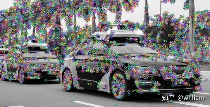
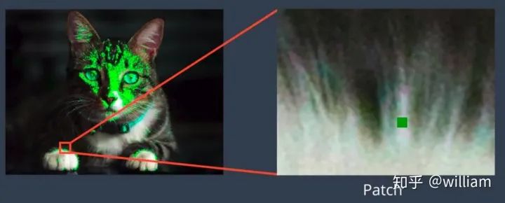
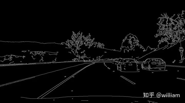
Features are pieces of information related to solving a computational task for a specific application. Features may be specific structures in an image, such as points, edges, or objects. Features may also be the results of general neighborhood operations or feature detection applied to the image. These features can be divided into two main categories:1. Features at specific locations in the image, such as peaks, building corners, doorways, or interestingly shaped snow blocks. These localized features are often referred to as keypoint features (or even corner points), and they are usually described by pixel blocks that appear around the point location, which are often referred to as image patches.2. Features that can be matched based on their direction and local appearance (edge contours) are called edges, which can also indicate object boundaries and occlusion events in image sequences.KeypointsEdges
Main Components of Feature Extraction and Matching
1. Detection: Identify interest points2. Description: Describe the local appearance around each feature point; this description is (ideally) invariant to changes in illumination, translation, scale, and in-plane rotation. We typically provide a descriptor vector for each feature point.3. Matching: Identify similar features by comparing descriptors in the images. For two images, we can obtain a set of pairs (Xi, Yi) -> (Xi’, Yi’), where (Xi, Yi) is a feature from one image, and (Xi’, Yi’) is a feature from another image.Detector
Keypoint/Interest Point
Keypoints, also known as interest points, are points expressed in texture. Keypoints are often points where the direction of object boundaries suddenly changes or the intersection between two or more edge segments. They have a clear position in image space or are well localized. Even in the presence of disturbances such as changes in illumination and brightness in the local or global image domain, keypoints remain stable and can be reliably computed repeatedly. Additionally, they should provide effective detection.There are two methods for computing keypoints:1. Based on image brightness (usually through image derivatives).2. Based on boundary extraction (usually through edge detection and curvature analysis).
Invariance of Keypoint Detectors to Photometric and Geometric Changes
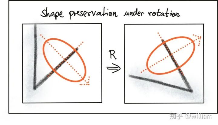
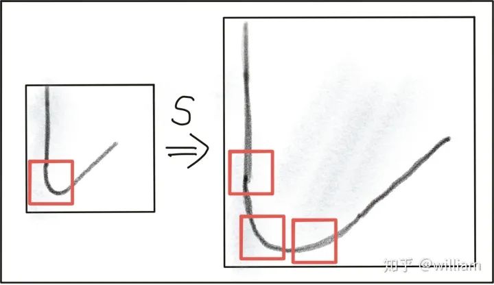
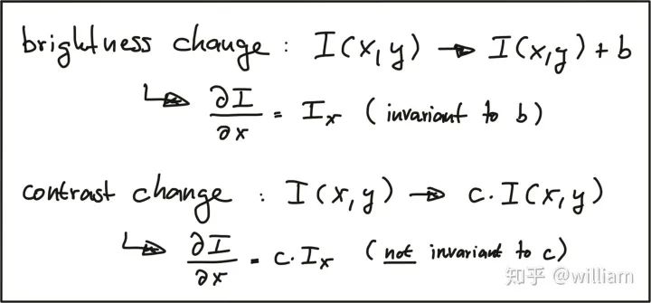
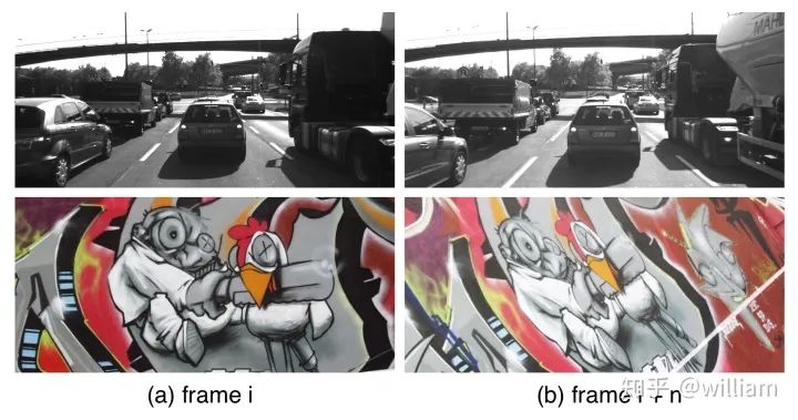
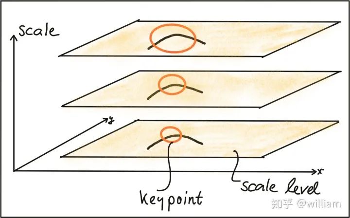
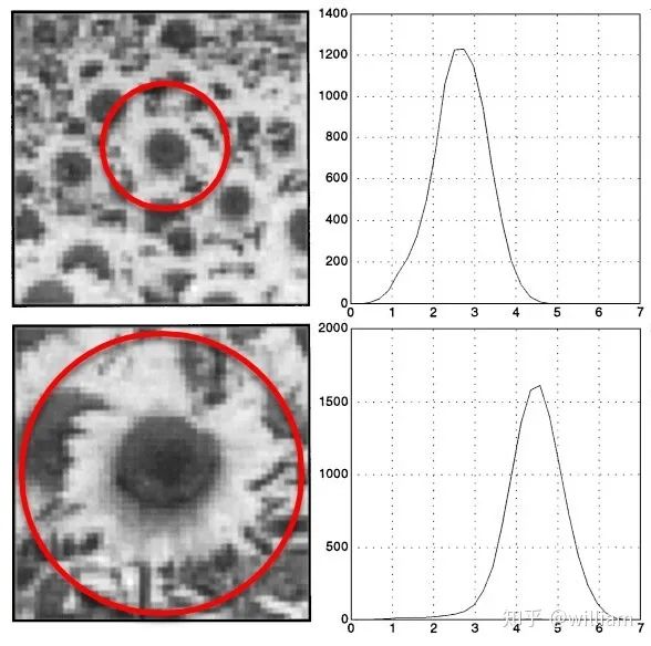
In the OPENCV library, we can choose from many feature detectors, and the choice of feature detector depends on the type of keypoints to be detected and the properties of the image, considering the robustness of the corresponding detector to photometric and geometric transformations.When selecting a suitable keypoint detector, we need to consider four basic types of transformations:1. Rotation Transformation2. Scale Transformation3. Intensity Transformation4. Affine TransformationThe graffiti sequence is one of the standard image sets used in computer vision, and we can observe that the i+n-th frame of the graffiti image includes all transformation types. For the highway sequence, when focusing on the vehicles in front, there are only scale and intensity changes between the i-th and i+n-th frames.The traditional HARRIS sensor has strong robustness under rotation and additive intensity offset, but is sensitive to scale changes, multiplicative intensity offset (i.e., contrast changes), and affine transformations.Automatic Scale SelectionTo detect keypoints at the ideal scale, we must know (or find) their respective dimensions in the image and adapt the size of the Gaussian window w(x,y) introduced earlier in this section. If the scale of the keypoints is unknown or if the keypoints exist in images of different sizes, detection must be performed continuously at multiple scales.Based on the standard deviation increment between adjacent layers, the same keypoint may be detected multiple times. This raises the issue of selecting the “correct” scale that best represents the keypoint. In 1998, Tony Lindeberg published a method called “Feature Detection with Automatic Scale Selection”. It proposed a function f(x,y,scale) that can be used to select keypoints that have stable maxima at scale FF. The scale that maximizes Ff is referred to as the “feature scale” of each keypoint.As shown in the figure below, such a function FF has been evaluated at several scale levels, and the second image shows a clear maximum, which can be viewed as the feature scale of the image content within a circular region.A good detector can automatically select the feature scale of keypoints based on the structural characteristics of the local neighborhood. Modern keypoint detectors typically have this capability, thus showing strong robustness to changes in image scale.
Common Keypoint Detectors
Keypoint detectors are a very popular research area, and many powerful algorithms have been developed over the years. Applications of keypoint detection include object recognition and tracking, image matching and panorama stitching, as well as robotic mapping and 3D modeling. The choice of detector not only requires comparing the invariance in the transformations mentioned above but also comparing the detection performance and processing speed of the detectors.
Classic Keypoint Detectors
The goal of classic keypoint detectors is to maximize detection accuracy, while complexity is generally not the primary consideration.
SURF – 2006 Speeded Up Robust Features (Bay, Tuytelaars, Van Gool) – None free
Modern Keypoint Detectors
In recent years, some faster detectors have been developed for real-time applications on smartphones and other portable devices. The list below shows the most popular detectors in this group:
FAST – 2006 Features from Accelerated Segment Test (FAST) (Rosten, Drummond)
BRIEF – 2010 Binary Robust Independent Elementary Features (BRIEF) (Calonder, et al.)
ORB – 2011 Oriented FAST and Rotated BRIEF (ORB) (Rublee et al.)
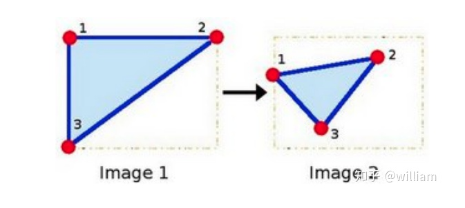
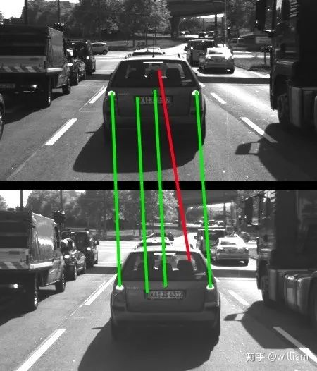
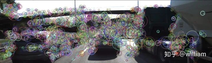
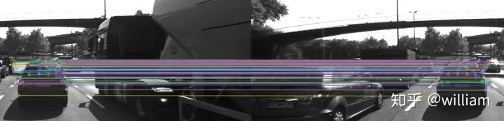
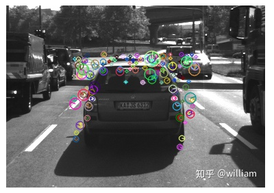
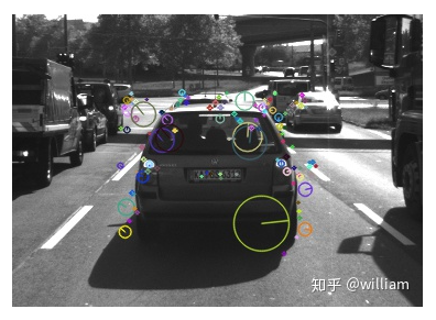
Since our task is to find corresponding keypoints in image sequences, we need a method based on similarity measures to reliably assign keypoints to one another. Many literatures have proposed various similarity measures (called Descriptors), and many authors have simultaneously released a new method for keypoint detection along with optimized similarity measures for their keypoint types. In other words, most of the OPENCV keypoint detection functions can also be used to generate keypoint descriptors.The difference is:Keypoint detectors are algorithms that select points from the image based on local maxima of functions, such as the “corner” measure we see in the HARRIS detector.Keypoint descriptors are vectors used to describe the pixel values of the image patches around keypoints. The description methods range from comparing raw pixel values to more complex methods, such as histograms of oriented gradients.Keypoint detectors generally find feature points from a frame image. Descriptors help us assign similar keypoints from different images to one another during the “keypoint matching” step. As shown in the figure below, a set of keypoints in one frame is assigned to keypoints in another frame to maximize the similarity of their respective descriptors, and these keypoints represent the same object in the image. Besides maximizing similarity, good descriptors should also minimize mismatches, i.e., avoid assigning keypoints that do not correspond to the same object to one another.
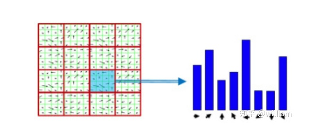
HOG Descriptor Based on Gradients
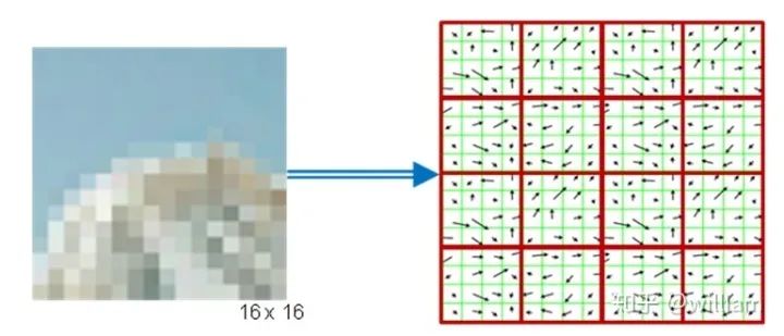
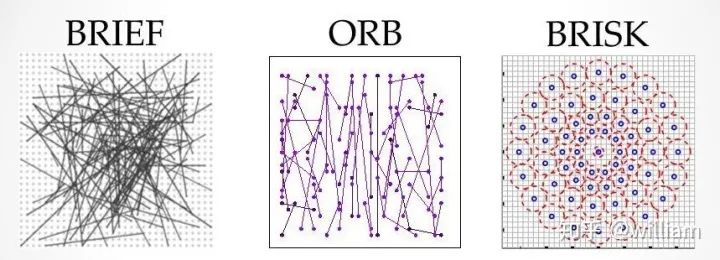
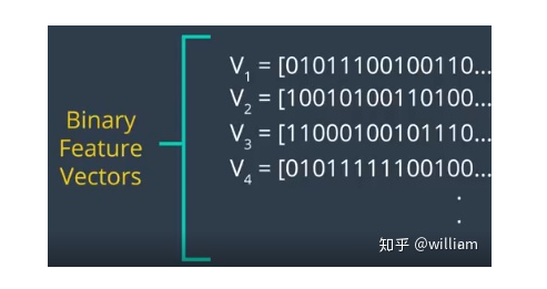
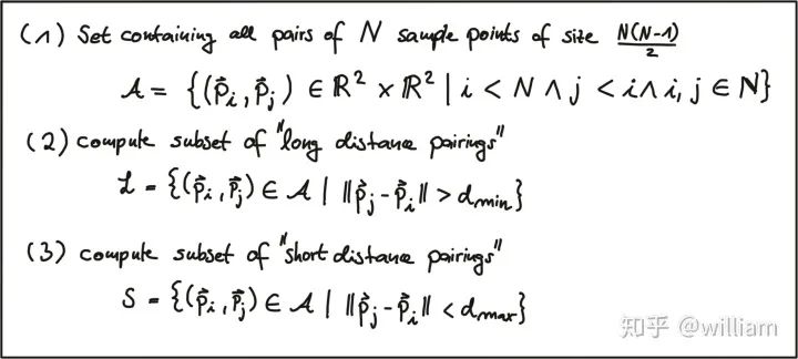
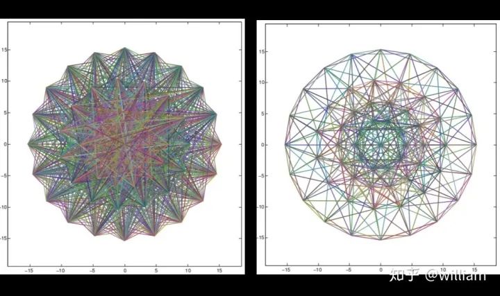
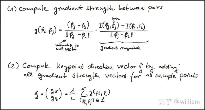
Although more and more fast detector/descriptor combinations have emerged, the Scale-Invariant Feature Transform (SIFT), which is based on Histogram of Oriented Gradients (HOG) descriptors, is still widely used. The basic idea of HOG is to describe the structure of objects based on the distribution of intensity gradients in the local neighborhood of the object. To achieve this, the image is divided into multiple cells, where gradients are computed and collected into histograms. Then, the histogram sets of all cells are used as similarity measures to uniquely identify image blocks or objects.SIFT/SURF uses HOG as descriptors, including both keypoint detectors and descriptors, which are very powerful but patented. SURF is an improvement on SIFT, which not only improves computational speed but also increases robustness; the implementation principles of both are quite similar. Here, I will only introduce SIFT.The SIFT method follows a five-step process, which will be briefly summarized below.First, keypoints in the image are detected using a method called “Laplacian of Gaussian (LoG)”, which is based on the second-order intensity derivative. LoG is applied at various scale levels of the image and tends to detect blobs rather than corners. In addition to using a unique scale level, directions are assigned to keypoints based on the intensity gradients in the local neighborhood around the keypoints.Second, for each keypoint, the surrounding area is changed by removing direction, ensuring a normalized direction. Additionally, the size of this area will be adjusted to 16 x 16 pixels, providing a standardized image patch.Third, the direction and magnitude of each pixel in the normalized image patch are calculated based on intensity gradients _Ix_ and _Iy_.Fourth, the normalized patches are divided into a grid of 4 x 4 cells. Within each cell, the directions of pixels that exceed a magnitude threshold are collected into a histogram consisting of 8 bins.Finally, all 16 cell histograms of 8 columns are concatenated into a 128-dimensional vector (descriptor) that uniquely represents the keypoint.The SIFT detector/descriptor can reliably identify objects even in clutter and partial occlusion. Uniform changes in scale, rotation, brightness, and contrast are invariant, and affine distortions are even invariant.The downside of SIFT is its low speed, which makes it impractical for real-time applications like smartphones. Other members of the HOG series (such as SURF and GLOH) have been optimized for speed. However, they are still computationally expensive and should not be used in real-time applications. Additionally, SIFT and SURF have many patents and cannot be freely used in commercial environments. To use SIFT in OpenCV, you must include #include <opencv2/xfeatures2d/nonfree.hpp>, and you need to install the OPENCV_contribute package, ensuring to enable OPENCV_ENABLE_NONFREE in Cmake options.Binary DescriptorsThe problem with HOG-based descriptors is that they rely on computing intensity gradients, which is a very expensive operation. Even though some improvements have been made (such as SURF), using integral images has increased speed, but these methods are still not suitable for real-time applications on devices with limited processing power (e.g., smartphones). The binary descriptor family offers a faster (free) alternative to HOG methods, but with slightly lower accuracy and performance.The core idea of binary descriptors is to rely solely on intensity information (i.e., the image itself) and encode the information around keypoints into a string of binary digits. When searching for corresponding keypoints, these digits can be compared very efficiently during the matching step. In other words, binary descriptors encode the information of interest points into a series of numbers and serve as a digital “fingerprint” that can be used to distinguish one feature from another. The most popular binary descriptors currently include BRIEF, BRISK, ORB, FREAK, and KAZE (all of which can be found in the OpenCV library).Binary DescriptorsFrom a high-level perspective, binary descriptors consist of three main parts:1. A sampling pattern that describes the location of sample points around the keypoint.2. A direction compensation method that eliminates the influence of rotation around the keypoint location.3. A method for selecting sample pairs that generates paired sample points that are compared based on their intensity values. If the first value is greater than the second value, we write a “1” in the binary string; otherwise, we write a “0”. After performing this on all pairs of sample points in the sampling pattern, a long binary chain (or “string”) is created (hence the name of the descriptor class family).BRISK “Binary Robust Invariant Scalable Keypoints” is a representative keypoint detector/descriptor of binary descriptors. Here, I will only introduce BRISK.In 2011, Stefan Leutenegger proposed BRISK, a combination of a FAST detector and a Binary descriptor created by sampling the intensity comparisons around each keypoint neighborhood.The sampling pattern of BRISK consists of multiple sampling points (in blue), where each sampling point is surrounded by concentric rings (in red) representing the area where Gaussian smoothing is applied. Unlike some other binary descriptors (such as ORB or Brief), the BRISK sampling pattern is fixed. Smoothing is critical to avoid aliasing (which causes different signals to become difficult to distinguish when sampled or overlap with one another).During the sample pair selection, the BRISK algorithm distinguishes between long-distance pairs and short-distance pairs. Long-distance pairs (i.e., sample points with minimal distance from each other in the sampling pattern) are used to estimate the direction of the image patch based on intensity gradients, while short-distance pairs are used for intensity comparisons to assemble the descriptor string. Mathematically, these pairs are represented as follows:First, we define the set A of all possible sampling point pairs. Then, we extract a subset L from A, where the Euclidean distance of subset L is greater than the upper threshold. L is used for estimating direction with long-distance pairs. Finally, we extract those pairs from A whose Euclidean distance is below the lower threshold. The set S contains short-distance pairs used to assemble the binary descriptor string.The figure below shows two types of distance pairs on the sampling pattern: short pairs (left) and long pairs (right).From the long pairs, the keypoint direction vector G is computed as follows:First, the gradient intensity between two sampling points is calculated based on normalized unit vectors, where the normalized unit vector gives the direction between the two points, multiplied by the intensity difference of the two points at their respective scales. Then in (2), the keypoint direction vector g is computed from the total of all gradient intensities.Based on g, we can rearrange the short-distance pairs using the direction of the sampling pattern to ensure rotation invariance. Based on rotation-invariant short-distance pairs, we can construct the final binary descriptor as follows:After calculating the orientation of the keypoint based on g, we use it to make the short-distance pairs rotation invariant. Then, the intensities S between all pairs are compared and used to assemble the binary descriptor for matching.OPENCV Detector/Descriptor ImplementationCurrently, there are various feature point detectors/descriptors, such as HARRIS, SHI-TOMASI, FAST, BRISK, ORB, AKAZE, SIFT, FREAK, BRIEF. Each of these deserves a blog post to describe individually, but the purpose of this article is to provide an overview, so I will not analyze these detectors/descriptors in detail from a theoretical perspective. There are many articles online describing these detectors/descriptors, but I still recommend that you first look at the OPENCV library’s Tutorial: How to Detect and Track Object With OpenCV.Next, I will introduce the code implementation and parameter details of each feature point detector/descriptor, and at the end of the article, I will evaluate these combinations based on practical results.Some OPENCV functions can be used for both detectors/descriptors, but some combinations may have issues.SIFT Detector/Descriptor SIFT detector and ORB descriptor do not work together
int nfeatures = 0; // The number of best features to retain. int nOctaveLayers = 3; // The number of layers in each octave. 3 is the value used in D. Lowe paper. double contrastThreshold = 0.04; // The contrast threshold used to filter out weak features in semi-uniform (low-contrast) regions. double edgeThreshold = 10; // The threshold used to filter out edge-like features. double sigma = 1.6; // The sigma of the Gaussian applied to the input image at the octave #0. xxx=cv::xfeatures2d::SIFT::create(nfeatures, nOctaveLayers, contrastThreshold, edgeThreshold, sigma);
HARRIS Detector
// Detector parameters int blockSize = 2; // for every pixel, a blockSize × blockSize neighborhood is considered int apertureSize = 3; // aperture parameter for Sobel operator (must be odd) int minResponse = 100; // minimum value for a corner in the 8bit scaled response matrix double k = 0.04; // Harris parameter (see equation for details) // Detect Harris corners and normalize output cv::Mat dst, dst_norm, dst_norm_scaled; dst = cv::Mat::zeros(img.size(), CV_32FC1); cv::cornerHarris(img, dst, blockSize, apertureSize, k, cv::BORDER_DEFAULT); cv::normalize(dst, dst_norm, 0, 255, cv::NORM_MINMAX, CV_32FC1, cv::Mat()); cv::convertScaleAbs(dst_norm, dst_norm_scaled); // Look for prominent corners and instantiate keypoints double maxOverlap = 0.0; // max. permissible overlap between two features in %, used during non-maxima suppression for (size_t j = 0; j < dst_norm.rows; j++) { for (size_t i = 0; i < dst_norm.cols; i++) { int response = (int) dst_norm.at<float>(j, i); if (response > minResponse) { // only store points above a threshold cv::KeyPoint newKeyPoint; newKeyPoint.pt = cv::Point2f(i, j); newKeyPoint.size = 2 * apertureSize; newKeyPoint.response = response; // perform non-maximum suppression (NMS) in local neighbourhood around new key point bool bOverlap = false; for (auto it = keypoints.begin(); it != keypoints.end(); ++it) { double kptOverlap = cv::KeyPoint::overlap(newKeyPoint, *it); if (kptOverlap > maxOverlap) { bOverlap = true; if (newKeyPoint.response > (*it).response) { // if overlap is >t AND response is higher for new kpt *it = newKeyPoint; // replace old key point with new one break; // quit loop over keypoints } } } if (!bOverlap) { // only add new key point if no overlap has been found in previous NMS keypoints.push_back(newKeyPoint); // store new keypoint in dynamic list } } } // eof loop over cols} // eof loop over rows
SHI-TOMASI Detector
int blockSize = 6; // size of an average block for computing a derivative covariation matrix over each pixel neighborhood double maxOverlap = 0.0; // max. permissible overlap between two features in % double minDistance = (1.0 - maxOverlap) * blockSize; int maxCorners = img.rows * img.cols / max(1.0, minDistance); // max. num. of keypoints double qualityLevel = 0.01; // minimal accepted quality of image corners double k = 0.04; bool useHarris = false; // Apply corner detection vector<cv::Point2f> corners; cv::goodFeaturesToTrack(img, corners, maxCorners, qualityLevel, minDistance, cv::Mat(), blockSize, useHarris, k); // add corners to result vector for (auto it = corners.begin(); it != corners.end(); ++it) { cv::KeyPoint newKeyPoint; newKeyPoint.pt = cv::Point2f((*it).x, (*it).y); newKeyPoint.size = blockSize; keypoints.push_back(newKeyPoint); }
BRISK Detector/Descriptor
int threshold = 30; // FAST/AGAST detection threshold score. int octaves = 3; // detection octaves (use 0 to do single scale) float patternScale = 1.0f; // apply this scale to the pattern used for sampling the neighbourhood of a keypoint. xxx=cv::BRISK::create(threshold, octaves, patternScale);
FREAK Detector/Descriptor
bool orientationNormalized = true; // Enable orientation normalization. bool scaleNormalized = true; // Enable scale normalization. float patternScale = 22.0f; // Scaling of the description pattern. int nOctaves = 4; // Number of octaves covered by the detected keypoints. const std::vector<int> &selectedPairs = std::vector<int>(); // (Optional) user-defined selected pairs indexes, xxx=cv::xfeatures2d::FREAK::create(orientationNormalized, scaleNormalized, patternScale, nOctaves,selectedPairs);
FAST Detector/Descriptor
int threshold = 30; // Difference between intensity of the central pixel and pixels of a circle around this pixel bool nonmaxSuppression = true; // perform non-maxima suppression on keypoints cv::FastFeatureDetector::DetectorType type = cv::FastFeatureDetector::TYPE_9_16; // TYPE_9_16, TYPE_7_12, TYPE_5_8 xxx=cv::FastFeatureDetector::create(threshold, nonmaxSuppression, type);
ORB Detector/Descriptor SIFT detector and ORB descriptor do not work together
int nfeatures = 500; // The maximum number of features to retain. float scaleFactor = 1.2f; // Pyramid decimation ratio, greater than 1. int nlevels = 8; // The number of pyramid levels. int edgeThreshold = 31; // This is size of the border where the features are not detected. int firstLevel = 0; // The level of pyramid to put source image to. int WTA_K = 2; // The number of points that produce each element of the oriented BRIEF descriptor. auto scoreType = cv::ORB::HARRIS_SCORE; // The default HARRIS_SCORE means that Harris algorithm is used to rank features. int patchSize = 31; // Size of the patch used by the oriented BRIEF descriptor. int fastThreshold = 20; // The fast threshold. xxx=cv::ORB::create(nfeatures, scaleFactor, nlevels, edgeThreshold, firstLevel, WTA_K, scoreType,patchSize, fastThreshold);
AKAZE Detector/Descriptor KAZE/AKAZE descriptors will only work with KAZE/AKAZE detectors.
auto descriptor_type = cv::AKAZE::DESCRIPTOR_MLDB; // Type of the extracted descriptor: DESCRIPTOR_KAZE, DESCRIPTOR_KAZE_UPRIGHT, DESCRIPTOR_MLDB or DESCRIPTOR_MLDB_UPRIGHT. int descriptor_size = 0; // Size of the descriptor in bits. 0 -> Full size int descriptor_channels = 3; // Number of channels in the descriptor (1, 2, 3) float threshold = 0.001f; // Detector response threshold to accept point int nOctaves = 4; // Maximum octave evolution of the image int nOctaveLayers = 4; // Default number of sublevels per scale level auto diffusivity = cv::KAZE::DIFF_PM_G2; // Diffusivity type. DIFF_PM_G1, DIFF_PM_G2, DIFF_WEICKERT or DIFF_CHARBONNIER xxx=cv::AKAZE::create(descriptor_type, descriptor_size, descriptor_channels, threshold, nOctaves,nOctaveLayers, diffusivity);
BRIEF Detector/Descriptor
int bytes = 32; // Length of the descriptor in bytes, valid values are: 16, 32 (default) or 64. bool use_orientation = false; // Sample patterns using keypoints orientation, disabled by default. xxx=cv::xfeatures2d::BriefDescriptorExtractor::create(bytes, use_orientation);
Descriptor MatchingFeature matching, or generally speaking, image matching, is part of computer vision applications such as image registration, camera calibration, and object recognition, and is the task of establishing correspondences between two images of the same scene/target. A common method for image matching is to detect a set of interest points associated with image descriptors from image data. Once features and descriptors are extracted from two or more images, the next step is to establish some preliminary feature matches between these images.Generally, the performance of feature matching methods depends on the nature of the underlying keypoints and the choice of associated image descriptors.We have learned that keypoints can be described by transforming their local neighborhoods into high-dimensional vectors, capturing unique features of gradient or intensity distributions.
Distance Between Descriptors
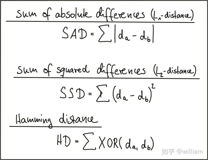
Feature matching requires calculating the distance between two descriptors, so that their differences are converted into a single number, which we can use as a simple measure of similarity.Currently, there are three distance metrics:
Sum of Absolute Differences (SAD) – L1-norm
Sum of Squared Differences (SSD) – L2-norm
Hamming Distance
The difference between SAD and SSD is that the shortest distance between the two is a straight line. Given the two components of each vector, SAD calculates the sum of length differences, which is a one-dimensional process. SSD, on the other hand, calculates the sum of squares, following the Pythagorean theorem in a right triangle, where the sum of the squares of the width sides equals the square of the hypotenuse. Therefore, in terms of the geometric distance between two vectors, L2-norm is a more accurate measure. Note that the same principle applies to high-dimensional descriptors.Hamming distance is well-suited for binary descriptors consisting solely of 1s and 0s, calculated by using the XOR function to compute the differences between two vectors; if two bits are the same, it returns zero; if the two bits are different, it returns 1. Thus, the total of all XOR operations is the number of differing bits between the two descriptors.It is worth noting that the appropriate distance metric must be chosen based on the type of descriptor used.
HOG descriptors: SIFT (and SURF and GLOH, all patented) – L2-norm
Finding Matching Pairs
Let’s assume there are N keypoints and their associated descriptors in one image, and M keypoints in another image.
Brute Force Matching
The most obvious way to find correspondences is to compare all features with one another, i.e., performing N x M comparisons. For a given keypoint in the first image, it will fetch each keypoint in the second image and calculate the distance. The keypoint with the smallest distance will be considered a pair. This method is called “Brute Force Matching” or “Nearest Neighbor Matching”. The output of brute force matching in OPENCV is a list of keypoint pairs, sorted by the distance of their descriptors under the selected distance function.
Fast Nearest Neighbor (FLANN)
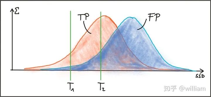
In 2014, David Lowe and Marius Muja released the “Fast Library for Approximate Nearest Neighbors (FLANN)”. FLANN trains an index structure to traverse potential matching candidates created using machine learning concepts. The library builds very efficient data structures (KD-trees) for searching matching pairs and avoids exhaustive search through brute force. Thus, it is faster, and the results are also very good, but it still requires tuning matching parameters.Both BFMatching and FLANN accept a descriptor distance threshold T, which is used to limit the number of matches to “good” and discard matches that do not correspond. The corresponding “good” pairs are referred to as “True Positives (TP)”, while incorrect pairs are referred to as “False Positives (FP)”. The task of choosing an appropriate value for T is to allow as many TP matches as possible while avoiding FP matches as much as possible. Depending on the image content and the corresponding detector/descriptor combinations, a balance must be found between TP and FP to reasonably balance the ratio between TP and FP. The figure below shows the distribution of TP and FP on SSD to illustrate threshold selection.The first threshold T1 is set as the maximum allowable SSD between two features, such that some correct positive matches are selected while almost completely avoiding incorrect positive matches. However, using this setting will also discard most TP matches. By increasing the matching threshold to T2, more TP matches can be selected, but the number of FP matches will also significantly increase. In practice, it is almost impossible to achieve a clear separation between TP and FP, so setting the matching threshold is always a trade-off between “good” and “bad” matches. Although it is usually impossible to avoid FP, the goal is always to minimize the number of FP as much as possible. Below are two strategies proposed to achieve this goal.
Selecting Matching Pairs
BFMatching – CrossCheck
As long as it does not exceed the selected threshold T, brute force matching will always return matches with keypoints even if there are no keypoints in the second image. This inevitably leads to many incorrect matches. One strategy to counter this situation is called Cross-Check Matching, which works by applying the matching process in both directions and only retaining those matches where the best match in one direction is the same as the best match in the other direction. The steps for the cross-checking method are:1. For each descriptor in the source image, find one or more best matches in the reference image.2. Switch the order of the source image and reference image.3. Repeat the matching process between the source image and reference image as in step 1.4. Select those keypoint pairs whose descriptors match best in both directions.Although cross-check matching increases processing time, it usually eliminates a large number of incorrect matches, so when accuracy is prioritized over speed, cross-checking should always be performed. Cross-checking is generally only used for BFMatching.
Nearest Neighbor Distance Ratio (NN)/K-Nearest Neighbor (KNN)
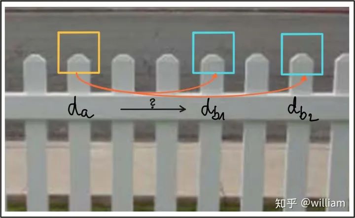
Another very effective method for reducing false positives is to calculate the nearest neighbor distance ratio for each keypoint.KNN differs from NN in that NN keeps only the best match for each feature point, while KNN keeps the k best matches (k=2) for each feature point.The main idea is not to apply the threshold directly to SSD. Instead, for each keypoint in the source image, the two (k=2) best matches are located in the reference image, and the ratio of the distances between the descriptors is calculated. Then, the threshold is applied to the ratio to filter out ambiguous matches. The figure below illustrates the principle.In this example, the image patch with descriptor da is compared with the other two image patches with descriptors d_b1 and d_b2. It can be seen that the image patches appear very similar and lead to ambiguity, thus being unreliable. By calculating the ratio of the best match to the second-best match, these weaker candidates can be filtered out.In practice, a threshold of 0.8 has been shown to provide a good balance between TP and FP. In the image sequences examined in the original SIFT, this setting can eliminate 90% of false matches while losing less than 5% of correct matches. Note that only KNN can set the threshold of 0.8. NN will only provide one best match.Below is the execution code for matching:
void matchDescriptors(std::vector<cv::KeyPoint> &kPtsSource, std::vector<cv::KeyPoint> &kPtsRef, cv::Mat &descSource, cv::Mat &descRef, std::vector<cv::DMatch> &matches, std::string descriptorclass, std::string matcherType, std::string selectorType) { // configure matcher bool crossCheck = false; cv::Ptr<cv::DescriptorMatcher> matcher; int normType; if (matcherType.compare("MAT_BF") == 0) { int normType = descriptorclass.compare("DES_BINARY") == 0 ? cv::NORM_HAMMING : cv::NORM_L2; matcher = cv::BFMatcher::create(normType, crossCheck); } else if (matcherType.compare("MAT_FLANN") == 0) { // OpenCV bug workaround : convert binary descriptors to floating point due to a bug in current OpenCV implementation if (descSource.type() !=CV_32F) { descSource.convertTo(descSource, CV_32F); // descRef.convertTo(descRef, CV_32F); } if (descRef.type() !=CV_32F) { descRef.convertTo(descRef, CV_32F); } matcher = cv::DescriptorMatcher::create(cv::DescriptorMatcher::FLANNBASED); } // perform matching task if (selectorType.compare("SEL_NN") == 0) { // nearest neighbor (best match) matcher->match(descSource, descRef, matches); // Finds the best match for each descriptor in desc1 } else if (selectorType.compare("SEL_KNN") == 0) { // k nearest neighbors (k=2) vector<vector<cv::DMatch>> knn_matches; matcher->knnMatch(descSource, descRef, knn_matches, 2); //-- Filter matches using the Lowe's ratio test double minDescDistRatio = 0.8; for (auto it = knn_matches.begin(); it != knn_matches.end(); ++it) { if ((*it)[0].distance < minDescDistRatio * (*it)[1].distance) { matches.push_back((*it)[0]); } } } }
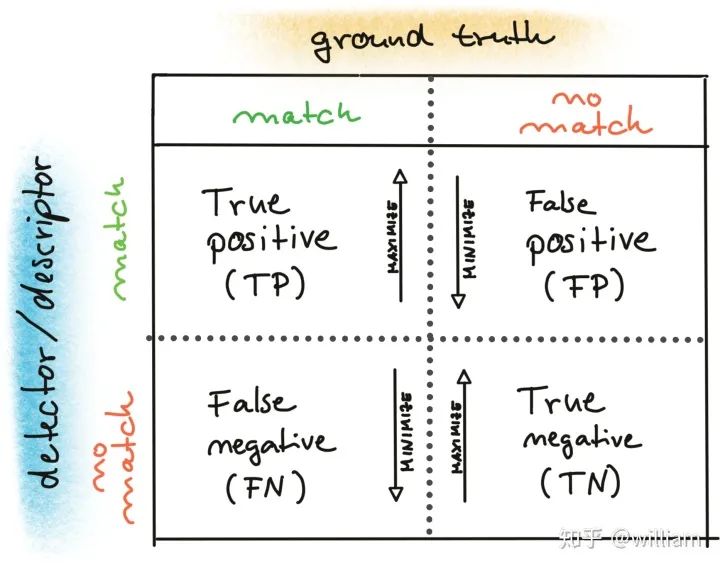
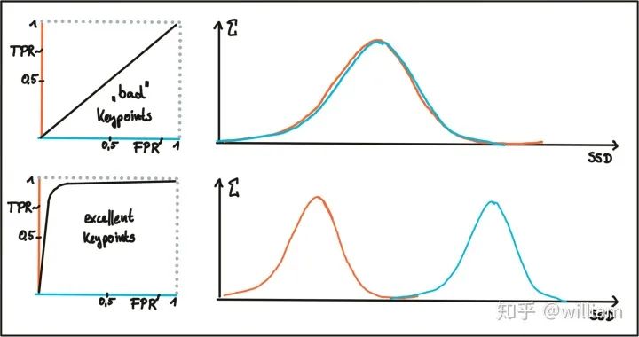
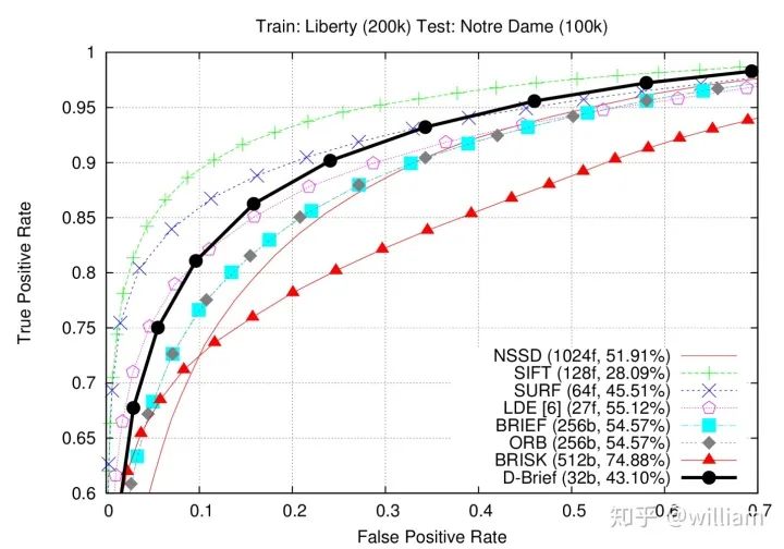
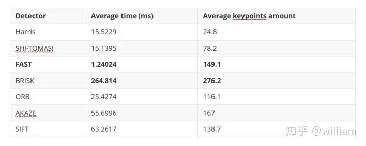
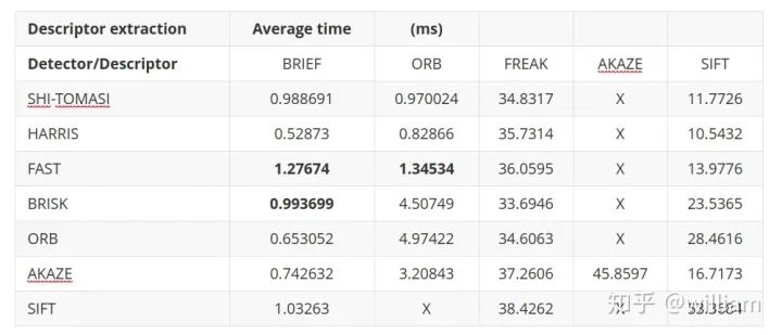
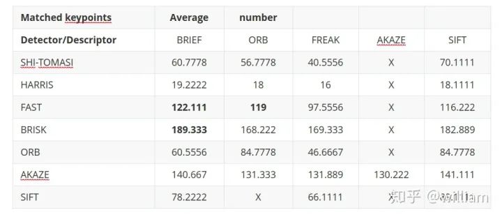
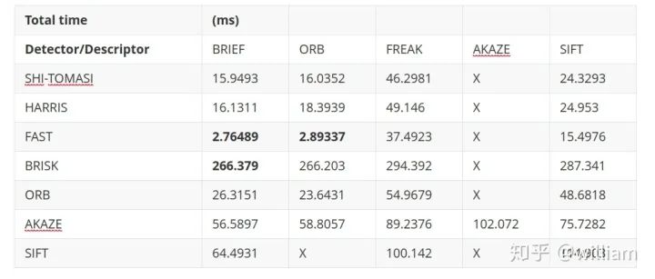
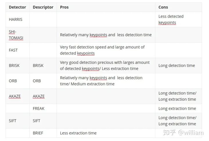
Evaluating Matching PerformanceCurrently, there are many types of detectors and descriptors for feature extraction and matching. To solve the problem, suitable algorithm pairs must be selected based on requirements such as the accuracy of keypoints or the number of matching pairs. Below, I outline the most commonly used measures.True Positive Rate (TPR) is the ratio of already matched correct keypoints (true positives – TP) to the total number of potential matches, including those missed by the detector/descriptor (false negatives – FN). A perfect matcher has a TPR of 1.0 because there will be no incorrect matches. TPR is also known as recall, and can be used to quantify how many possible correct matches were actually discovered.False Positive Rate (FPR) is the ratio of already matched incorrect keypoints (false positives – FP) to all feature points that should not be matched. A perfect matcher has an FPR of 0.0. FPR is also known as false alarm rate, which describes the likelihood of the detector/descriptor selecting incorrect keypoint pairs.Matcher Precision is the number of correctly matched keypoints (TP) divided by the total number of matches. This measure is also known as the inlier ratio.Many people often have misconceptions about TP, FP, FN, and TN, especially FN and TN. The figure below defines each of them:Here, we need to introduce the definition of ROC.The ROC curve is a graphical chart that shows how well a detector/descriptor can distinguish between true and false matches as its discrimination threshold varies. ROC can visually compare different detectors/descriptors and select an appropriate discrimination threshold for each detector.The figure below shows how to construct the ROC by changing the discrimination threshold of SSD, based on the distribution of true positives and false positives. An ideal detector/descriptor has a TPR of 1.0, while the FPR is close to 0.0.The figure below shows examples of two good and bad detectors/descriptors. In the first example, it is impossible to safely distinguish between TP and FP because the two curves match, and changing the discrimination threshold will affect them in the same way. In the second example, the TP and FP curves do not overlap significantly, allowing for the selection of an appropriate discriminator threshold.In this figure, you can see the ROC curves of different descriptors (e.g., SIFT, BRISK, and several others) and visually compare them. Note that these results are only valid for the image sequences actually used for comparison – for other image sets (e.g., traffic scenes), results may vary significantly.ConclusionThe purpose of the 2D_Feature_Tracking project is to calculate the number of keypoints within the range of the vehicles ahead, detection time, description time, matching time, and the number of matched keypoints using all possible combinations of detectors and descriptors for all 10 images. In the matching step, the BF method and KNN selector are used, and the descriptor distance ratio is set to 0.8.Below are the results:Average detection time and number of keypoints detected for different detectorsDescription time for different detector and descriptor combinationsNumber of matched points for different detector and descriptor combinations (controlling the matching algorithm for invariants)Total runtime for different detector and descriptor combinationsFrom the first impression in the above table, it can be seen:Considering all these variations, I can say that the top three combinations of detectors/descriptors are:
FAST + BRIEF (Higher speed and relatively good accuracy)
BRISK + BRIEF (Higher accuracy)
FAST + ORB (relatively good speed and accuracy)
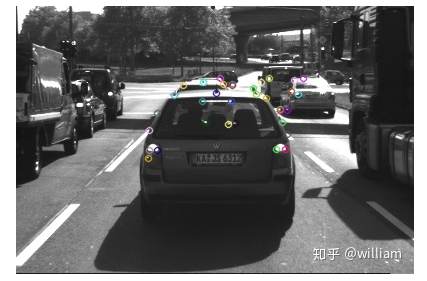
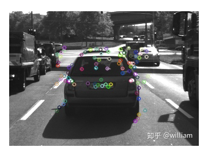
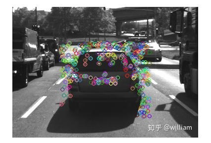
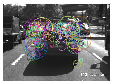
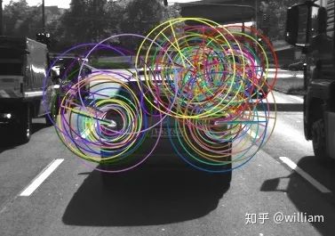
The above conclusions are based on the comparison of surface data from practical tests. You can also try modifying the combinations of detectors and descriptors in my code repository to see what different results you get.Finally, I quote Shaharyar Ahmed Khan Tareen’s conclusion in his paper “A Comparative Analysis of SIFT, SURF, KAZE, AKAZE, ORB, and BRISK” comparing the performance of different detector and descriptor combinations:SIFT, SURF, and BRISK are considered to be the most scale-invariant feature detectors (based on repeatability), which are unaffected by a wide range of scale variations. ORB has the least scale invariance. ORB (1000), BRISK (1000), and AKAZE have higher rotation invariance than others. Compared to the others, ORB and BRISK are generally more invariant to affine changes. SIFT, KAZE, AKAZE, and BRISK have higher image rotation accuracy than the rest. Although ORB and BRISK are the most efficient algorithms for detecting a large number of features, the matching time for such a large number of features prolongs the overall image matching time. In contrast, ORB (1000) and BRISK (1000) perform the fastest image matching, but their accuracy suffers. For all types of geometric transformations, SIFT and BRISK have the highest overall accuracy, with SIFT being considered the most accurate algorithm.Quantitative comparisons indicate the general order of the ability of feature detectors and descriptors to detect a large number of features as:ORB > BRISK > SURF > SIFT > AKAZE > KAZEThe order of computational efficiency for each feature point’s feature detection descriptor is:ORB > ORB (1000) > BRISK > BRISK (1000) > SURF (64D) > SURF (128D) > AKAZE > SIFT > KAZEThe order of effective feature matching for each feature point is:ORB (1000) > BRISK (1000) > AKAZE > KAZE > SURF (64D) > ORB > BRISK > SIFT > SURF (128D)The order of overall image matching speed for feature detection descriptors is:ORB (1000) > BRISK (1000) > AKAZE > KAZE > SURF (64D) > SIFT > ORB > BRISK > SURF (128D)Note: The detected images from different detectors show the size and distribution of their keypoint neighborhoods.HARRISShi-TomasiFASTBRISIKORBAKAZESIFTReferencesUDACITYA Comparative Analysis of SIFT, SURF, KAZE, AKAZE, ORB, and BRISKDeepanshu Tyagi If you want to understand the entire process of image feature extraction and matching, you can refer to the README file in my code repository.If you have any questions, feel free to contact my personal email.Github: https://github.com/williamhyin/SFND_2D_Feature_TrackingEmail: [email protected]Linkedin: https://linkedin.com/in/williamhyinDownload 1: OpenCV-Contrib Extension Module Chinese TutorialReply in the background of the “Visual Learning for Beginners” public account:Chinese Tutorial for Extension Module, to download the first Chinese version of the OpenCV extension module tutorial on the internet, covering installation of extension modules, SFM algorithms, stereo vision, object tracking, biological vision, super-resolution processing, and more than twenty chapters.Download 2: Python Visual Practical Projects 52 LecturesReply in the background of the “Visual Learning for Beginners” public account:Python Visual Practical Projects, to download 31 visual practical projects including image segmentation, mask detection, lane detection, vehicle counting, eyeliner addition, license plate recognition, character recognition, emotion detection, text content extraction, facial recognition, etc., to help quickly learn computer vision.Download 3: OpenCV Practical Projects 20 LecturesReply in the background of the “Visual Learning for Beginners” public account:OpenCV Practical Projects 20 Lectures, to download 20 practical projects based on OpenCV to achieve advanced learning in OpenCV.
Discussion Group
Welcome to join the reader group of the public account to exchange with peers. Currently, there are WeChat groups for SLAM, 3D Vision, Sensors, Autonomous Driving, Computational Photography, Detection, Segmentation, Recognition, Medical Imaging, GAN, Algorithm Competitions, etc. (will gradually be subdivided in the future), please scan the WeChat number below to join the group, and note: “Nickname + School/Company + Research Direction”, for example: “Zhang San + Shanghai Jiao Tong University + Visual SLAM”. Please follow the format for notes, otherwise, it will not be approved. After successful addition, you will be invited to relevant WeChat groups based on research direction. Please do not send advertisements in the group, otherwise, you will be removed from the group. Thank you for your understanding~