Comprehensive Overview of CNN Algorithm Model

Hello everyone, today we will talk about CNN.

In simple terms, Convolutional Neural Networks (CNNs) are deep learning models particularly suited for processing image data. CNN consists of multiple layers of neural networks, each performing specific processing on the input data, ultimately outputting a classification result or other objectives.

Imagine you are looking at an image. You would first notice the overall outline and color, and then gradually focus on the details, such as edges and features. The working principle of CNN is somewhat similar to the human eye. It first detects basic features in the image, such as edges and corners, through the “convolutional layer,” and then progressively detects more complex features until it finally recognizes the entire object.

Algorithm Overview

Main Components

1. Convolutional Layer:

• Function: Detect basic features in the image.
• Analogy: Just like when you look at an image, you first notice the general shape and edges.

• Function: Reduce the amount of data while retaining important features.
• Analogy: When you look at an image, you ignore some details and focus only on the main parts.

• Function: Classify the extracted features.
• Analogy: Judging what the object in the image is based on the features you see.

• Function: Introduce non-linearity to the model, allowing it to handle complex data.
• Analogy: The process of information processing in the brain.

In summary:

• Convolutional Neural Networks are deep learning models that effectively process image data.
• They achieve understanding and classification of images by progressively extracting features from simple to complex.
• The structure of CNN is similar to how humans view images, understanding image content gradually from whole to detail.

Theoretical Foundation

The mathematical principles and algorithm flow of CNN involve multi-layer neural networks and some unique operations, such as convolution, pooling, and fully connected layers.

Mathematical Principles

1. Convolution:

The convolution operation is the core of CNN, used to extract local features of the image.

• Input: The input image (or feature map) is represented as a matrix.
• Kernel: A small matrix, also known as a filter or weight matrix.
• Output: Output feature map.

The formula for the convolution operation:

where is the pixel value at the current position in the input image, and is the weight in the convolution kernel.

2. Activation Function:

After convolution, a non-linear activation function is applied to introduce non-linear characteristics.

• The commonly used activation function is ReLU (Rectified Linear Unit):

3. Pooling:

The pooling layer is used to reduce the size of the feature map, thereby reducing computational load and preventing overfitting.

• Max Pooling:

where is the size of the pooling window.

• Average Pooling:

4. Fully Connected Layer:

The fully connected layer flattens the pooled feature map into a one-dimensional vector for classification or regression.

• Input: The output feature map from the previous layer is flattened into a one-dimensional vector.
• Weights: The weight matrix of the fully connected layer and the bias vector.
• Output: The output is obtained through linear transformation and activation function.

5. Loss Function: It calculates the difference between the predicted output and the actual labels to guide model training.

• For classification problems, the commonly used loss is cross-entropy:

where is the true label, and is the predicted probability.

Algorithm Flow

1. Input Image:

• Input an image (or a small batch of images), each represented as a matrix.

• Select multiple convolutional kernels (filters) to perform convolution operations on the input image, obtaining multiple feature maps.
• Apply activation functions (like ReLU) for non-linear transformation on each feature map.

• Perform pooling operations (like max pooling or average pooling) on the feature maps to reduce their size.

• Repeatedly apply convolutional and pooling layers to progressively extract higher-level features.

• Flatten the output from the last pooling layer into a one-dimensional vector to input into the fully connected layer.

• Through one or more fully connected layers, perform linear transformations and non-linear activations on the flattened features.
• The final layer outputs the probability distribution of categories or regression values.

• Use the loss function to calculate the difference between the predicted output and the actual labels.

• Update the weights of the convolutional kernels and fully connected layers using the gradient of the loss function through backpropagation.

• Through multiple iterations (epochs), perform the above process on the training dataset, continuously optimizing the model’s weights until the loss function converges or reaches the preset training count.

Convolutional Neural Networks extract local features of images through convolution layers, reduce data volume through pooling layers, and perform final classification or regression through fully connected layers. The entire process is trained and optimized through backpropagation and gradient descent algorithms. The structure of CNN enables it to perform excellently in image processing and computer vision tasks.

Application Scenarios

Applicable Problems

Convolutional Neural Networks (CNNs) are particularly suitable for handling the following types of problems:

1. Image Classification: Identifying and classifying the main objects in an image. For example, recognizing whether an image is of a cat or a dog.
2. Object Detection: Locating and labeling multiple objects in an image. For example, detecting pedestrians, vehicles, etc., in an image.
3. Image Segmentation: Dividing an image into multiple parts or objects. For example, segmenting tumor areas in medical images.
4. Facial Recognition: Identifying faces and performing identity verification. For example, automatic tagging features in social media.
5. Image Generation and Repair: Generating new images or repairing damaged images. For example, generating artworks through Generative Adversarial Networks (GANs).

Advantages

1. Automatic Feature Extraction: CNN automatically extracts features from images without needing manually designed features.
2. Weight Sharing: Convolution kernels share weights across the entire image, reducing the number of parameters and improving training efficiency.
3. Local Connectivity: Only focusing on local connections reduces computational load, making it suitable for handling large images.
4. Powerful Expressiveness: CNN can extract multi-level features when processing complex image data, performing excellently.

Disadvantages

1. Requires Large Amounts of Data: Training CNN requires a large amount of labeled data; insufficient data can lead to overfitting.
2. High Computational Resource Requirements: Training CNN requires significant computational resources (like GPUs), leading to longer training times.
3. Difficult to Interpret: The convolution kernels and activation values within CNN are challenging to interpret, resulting in low model interpretability.
4. Complex Hyperparameter Tuning: Selecting appropriate convolution kernel sizes, pooling methods, and network depths requires extensive experimentation and experience.

Prerequisites for Application

1. Ample Data: Requires a large number of labeled image data for training.
2. Computational Resources: Requires high-performance computing devices (like GPUs) for model training and prediction.
3. Data Preprocessing: Requires preprocessing of image data, such as normalization and data augmentation.
4. Appropriate Framework: Requires the use of deep learning frameworks (like TensorFlow, PyTorch) to implement and train models.

Real Application Cases

1. Image Classification:

• ImageNet: A large-scale image classification competition where CNN models (like AlexNet, ResNet) performed excellently.
• Google Photos: Automatically classifies and tags user-uploaded photos.

• Autonomous Driving: For example, Tesla’s autonomous driving system uses CNN to detect pedestrians, vehicles, and traffic signs on the road.
• Security Monitoring: Uses CNN to detect suspicious activities in surveillance videos.

• Medical Image Analysis: Uses CNN to segment tumor areas in CT or MRI images, improving diagnostic accuracy.
• Automatic Labeling: For example, segmenting different terrain areas in geographic images taken by drones.

• Social Media: For example, Facebook’s automatic facial recognition and tagging features.
• Security Systems: For example, facial recognition verification systems in airports and banks.

• Generative Adversarial Networks (GANs): For example, generating realistic human face images.
• Image Repair: For example, repairing damaged historical photographs or movie frames.

The powerful image processing capabilities of CNN make it the preferred model for many practical problems.

Complete Case Study

Here we will use a classic case to demonstrate the application of Convolutional Neural Networks (CNN).

1. Use the CIFAR-10 dataset for image classification.
2. Enhance visualization, including loss and accuracy curves during training, and visualize some prediction results.
3. Perform algorithm optimization, including hyperparameter tuning and advanced techniques like data augmentation and regularization.

First, here are the libraries we need:

import tensorflow as tf
from tensorflow.keras import datasets, layers, models
import matplotlib.pyplot as plt
import numpy as np

Load and Preprocess Data

We will use the CIFAR-10 dataset, which contains 60,000 32×32 color images, divided into 10 classes.

# Load CIFAR-10 dataset
(train_images, train_labels), (test_images, test_labels) = datasets.cifar10.load_data()

# Normalize pixel values to between 0-1
train_images, test_images = train_images / 255.0, test_images / 255.0

# Define class names
class_names = ['airplane', 'automobile', 'bird', 'cat', 'deer', 
               'dog', 'frog', 'horse', 'ship', 'truck']

Build Convolutional Neural Network

We will build a CNN with multiple convolutional and pooling layers and add Dropout to prevent overfitting.

model = models.Sequential()
model.add(layers.Conv2D(32, (3, 3), activation='relu', input_shape=(32, 32, 3)))
model.add(layers.MaxPooling2D((2, 2)))
model.add(layers.Conv2D(64, (3, 3), activation='relu'))
model.add(layers.MaxPooling2D((2, 2)))
model.add(layers.Conv2D(64, (3, 3), activation='relu'))
model.add(layers.Flatten())
model.add(layers.Dense(64, activation='relu'))
model.add(layers.Dropout(0.5))  # Add Dropout layer
model.add(layers.Dense(10))

Compile and Train Model

Compile the model using the Adam optimizer and sparse categorical cross-entropy loss function, then train it.

model.compile(optimizer='adam',
              loss=tf.keras.losses.SparseCategoricalCrossentropy(from_logits=True),
              metrics=['accuracy'])

history = model.fit(train_images, train_labels, epochs=20, 
                    validation_data=(test_images, test_labels))

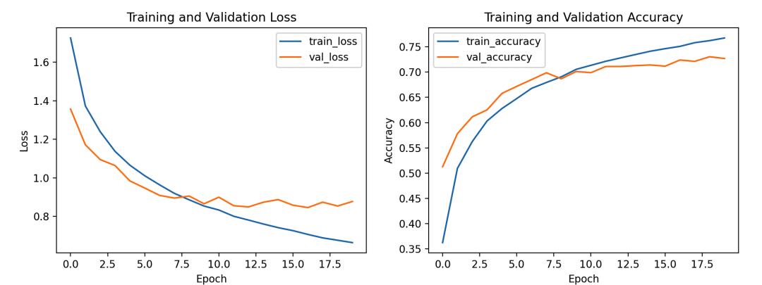
Visualize Training Process

We plot the loss and accuracy curves for training and validation.

plt.figure(figsize=(12, 4))

plt.subplot(1, 2, 1)
plt.plot(history.history['loss'], label='train_loss')
plt.plot(history.history['val_loss'], label='val_loss')
plt.xlabel('Epoch')
plt.ylabel('Loss')
plt.legend()
plt.title('Training and Validation Loss')

plt.subplot(1, 2, 2)
plt.plot(history.history['accuracy'], label='train_accuracy')
plt.plot(history.history['val_accuracy'], label='val_accuracy')
plt.xlabel('Epoch')
plt.ylabel('Accuracy')
plt.legend()
plt.title('Training and Validation Accuracy')

plt.show()

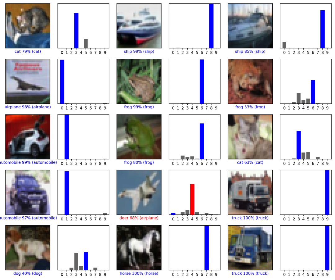
Display Some Prediction Results

This code will display some test images along with their predicted labels.

def plot_image(i, predictions_array, true_label, img):
    true_label, img = true_label[i], img[i]
    plt.grid(False)
    plt.xticks([])
    plt.yticks([])
    plt.imshow(img, cmap=plt.cm.binary)

    predicted_label = np.argmax(predictions_array)
    if predicted_label == true_label:
        color = 'blue'
    else:
        color = 'red'

    plt.xlabel("{} {:2.0f}% ({})".format(class_names[predicted_label],
                                         100*np.max(predictions_array),
                                         class_names[true_label[0]]),
                                         color=color)

def plot_value_array(i, predictions_array, true_label):
    true_label = true_label[i]
    plt.grid(False)
    plt.xticks(range(10))
    plt.yticks([])
    thisplot = plt.bar(range(10), predictions_array, color="#777777")
    plt.ylim([0, 1])
    predicted_label = np.argmax(predictions_array)

    thisplot[predicted_label].set_color('red')
    thisplot[true_label[0]].set_color('blue')

# Predict on test set
probability_model = tf.keras.Sequential([model, tf.keras.layers.Softmax()])
predictions = probability_model.predict(test_images)

# Display the first 15 test images, predicted labels, and true labels
num_rows = 5
num_cols = 3
num_images = num_rows*num_cols
plt.figure(figsize=(2*2*num_cols, 2*num_rows))
for i in range(num_images):
    plt.subplot(num_rows, 2*num_cols, 2*i+1)
    plot_image(i, predictions[i], test_labels, test_images)
    plt.subplot(num_rows, 2*num_cols, 2*i+2)
    plot_value_array(i, predictions[i], test_labels)
plt.tight_layout()
plt.show()

Algorithm Optimization

1. Data Augmentation:

   Data augmentation techniques can be used to increase the diversity of training data and reduce overfitting.

from tensorflow.keras.preprocessing.image import ImageDataGenerator

datagen = ImageDataGenerator(
    rotation_range=20,
    width_shift_range=0.2,
    height_shift_range=0.2,
    horizontal_flip=True,
)

datagen.fit(train_images)

1. Adjust Learning Rate: Use a learning rate scheduler to dynamically adjust the learning rate.

def scheduler(epoch, lr):
    if epoch < 10:
        return lr
    else:
        return lr * tf.math.exp(-0.1)

callback = tf.keras.callbacks.LearningRateScheduler(scheduler)

history = model.fit(datagen.flow(train_images, train_labels, batch_size=64),
                    epochs=50, validation_data=(test_images, test_labels),
                    callbacks=[callback])

From theory to the final case, everyone can build a simple CNN model and perform an image classification task, applying it to their own experiments.

Recently, I have prepared 16 major sections summarizing 124 algorithm problems, a complete machine learning booklet available for free~

Additionally, today I have prepared a collection of papers on Deep Learning, summarizing core papers from previous issues to share with everyone.

Click on the card and reply with “Deep Learning Papers” to get it~

If you are interested in articles like this.

Feel free to follow, like, and share~