Selected from Medium
Translated by Machine Heart
Contributors: Jiang Siyuan, Huang Xiaotian, Wu Pan
Image classification is one of the fundamental research topics in artificial intelligence, and researchers have developed a large number of algorithms for image classification. Recently, Shiyu Mou published an article on Medium that experimentally compared five methods for image classification (KNN, SVM, BP neural networks, CNN, and transfer learning). The related datasets and code for this research have also been published on GitHub.
Project address: https://github.com/Fdevmsy/Image_Classification_with_5_methods
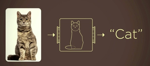
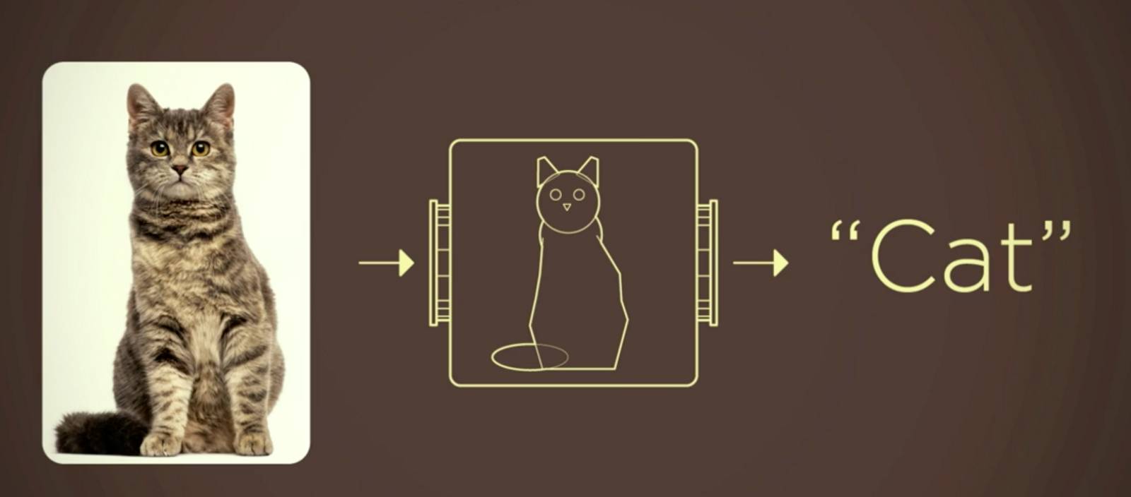
Image classification, as the name suggests, is about labeling input images with fixed categories. This is one of the core problems in the field of computer vision. Although it sounds simple, image classification has a large number of different practical applications.
Traditional Methods: Feature Description and Detection
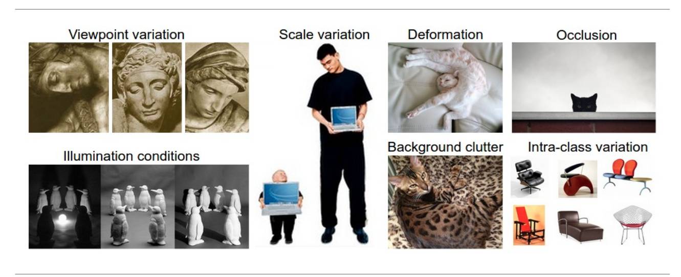
It may be beneficial for some sample tasks, but the reality is much more complex.
Therefore, we do not directly specify the visual appearance of each type through code, but instead use machine learning—providing the computer with many instances of each category, then developing learning algorithms to observe these instances and learn the appearance of each category.
However, image classification is so complex that deep learning models, such as CNN (Convolutional Neural Networks), are often used for processing. We already know that many algorithms we learn in class (such as KNN, SVM) are usually good at data mining; however, they are not the best choice for image classification.
Therefore, we will compare the algorithms learned in class with CNN and transfer learning.
Goals
Our goals are:
1. To compare KNN, SVM, BP neural networks with industry-standard algorithms for image recognition—CNN and transfer learning.
2. To gain experience in deep learning.
3. To explore machine learning frameworks through TensorFlow.
System Design & Implementation Details
Algorithms and Tools
The five methods used in this project are KNN, SVM, BP neural networks, CNN, and transfer learning.
The entire project can be divided into three categories of methods:
-
First category: using classroom algorithms such as KNN, SVM, BP neural networks. These algorithms are powerful and easy to implement. We mainly use sklearn to implement these algorithms.
-
Second category: Although traditional multi-layer perceptron models have been successfully applied to image recognition, they encounter dimensionality issues due to their fully connected nature, which prevents them from scaling well to higher resolution images. Therefore, we built a CNN using the deep learning framework TensorFlow.
-
Third category: Retraining the last layer of a pre-trained deep neural network called Inception V3, also provided by TensorFlow. Inception V3 was trained for the ImageNet Large Visual Recognition Challenge using data from 2012. This is a conventional task in computer vision, where the model attempts to classify all images into 1000 categories, such as zebras, dalmatian dogs, and dishwashers. To retrain this pre-trained network, we need to ensure that our dataset is not included in the pre-training.
Implementation
First category: Preprocess the dataset and implement KNN, SVM, BP neural networks using sklearn.
First, we defined two different preprocessing functions using the OpenCV package: the first is from image to feature vector, which can resize images and convert images into row pixel lists; the second is to extract color histograms, i.e., using cv2.normalize to extract a 3D color histogram from the HSV color space and flatten the result.
Next, we constructed several parameters that we need to parse. Since we want to test the accuracy of both the entire dataset and sub-datasets with different numbers of labels, we constructed a dataset as parameters and parsed it into our program. We also constructed the number of neighbors for the k-NN method as a parsing parameter.
After that, we began to extract features from each image in the dataset and put them into an array. We used cv2.imread to read each image and split the labels by extracting strings from the image names. In our dataset, we used the same format—category label.image number.jpg—to set names, so we could easily extract the classification labels of each image. Then we used these two functions to extract two types of features and append them to the array rawImages, while the previously extracted labels were appended to the array labels.
The next step is to split the dataset using the function train_test_split imported from the sklearn package. This set has the suffix RI, RL is the split result of rawImages and labels, and the other is the split result of features and labels. We used 85% of the dataset as the training set and the remaining 15% as the test set.
Finally, we applied KNN, SVM, and BP neural network functions to evaluate the data. For KNN we used KNeighborsClassifier, for SVM we used SVC, and for BP neural networks we used MLPClassifier.
Second category: Build CNN using TensorFlow. The entire purpose of TensorFlow is to allow you to build a computation graph (using languages like Python), and then execute that graph in C++ (which is more efficient than Python for the same computation load).
TensorFlow can also automatically compute the gradients needed to optimize graph variables, allowing the model to perform better. This is because the graph is composed of simple mathematical expressions, so the gradients of the entire graph can be computed using the chain rule of derivatives.
A TensorFlow graph consists of the following parts, each of which will be detailed below:
-
Placeholder variables for inputting data into the graph.
-
Optimization vectors to improve the convolutional network’s performance.
-
The mathematical formulas for the convolutional network.
-
Cost metrics that can guide variable optimization.
-
Optimization methods for updating variables.
-
The CNN architecture consists of a stack of different layers that transform the input into output through differentiable functions.
Therefore, in our implementation, the first layer is for storing images, then we constructed three convolutional layers using 2 x 2 max pooling and rectified linear unit (ReLU). The input is a 4D tensor:
-
Image number.
-
Y-axis of each image.
-
X-axis of each image.
-
Channel of each image.
The output is another 4D tensor:
-
Image number, same as input.
-
Y-axis of each image. If using 2×2 pooling, then the height and width of the input image are divided by 2.
-
X-axis of each image. Same as above.
-
Channels generated by convolutional filters.
Next, we constructed two fully connected layers at the end of the network. The input is a 2D shape tensor [num_images, num_inputs]. The output is also a 2D shape tensor [num_images, num_outputs].
However, to connect the convolutional layers and fully connected layers, we need a flatten layer to reduce the 4D vector to a 2D vector that can be input into the fully connected layer.
The end of a CNN is usually a softmax layer, which normalizes the outputs from the fully connected layer, thus each element is restricted between 0 and 1, and all elements sum to 1.
To optimize training results, we need a cost metric and minimize the cost in each iteration. The cost function we use here is cross-entropy (tf.nn.softmax_cross_entropy_with_logits()), and we take the average of cross-entropy across all image classifications. The optimization method is tf.train.AdamOptimizer(), which is a high-level form of gradient descent. This is a tunable parameter learning rate.
Third method: Retrain Inception V3. Modern object recognition models have millions of parameters and may take weeks to fully train a model. Transfer learning is a method that uses a pre-trained model from a classification dataset (like ImageNet) to complete this task quickly, as it only requires retraining the weights for new categories. Although such models do not perform as well as fully trained models, they are very efficient for many applications because they do not require a GPU and can complete training on a laptop in half an hour.
Readers can click the link to learn more about the training process of transfer learning: https://www.tensorflow.org/tutorials/image_retraining
First, we need to obtain the pre-trained model and remove the old top layer of the neural network, and then retrain an output layer based on our dataset. Although not all breeds of cats are represented in the original ImageNet dataset and fully trained models, the magic of transfer learning is that it can leverage the lower-level features that the pre-trained model has learned to recognize certain objects, as these lower-level features can be applied to many recognition tasks without modification. Then we analyze all local images and calculate the bottleneck values for each. Since each image is reused multiple times during training, calculating each bottleneck value takes a lot of time, but we can speed up this process by caching these bottleneck values, thus avoiding repeated calculations.
This script will run 4000 training steps. Each step randomly selects 10 images from the training set and searches for their bottleneck values from the cache, then trains them through the last layer to get predictions. These predictions will update the weights of the last layer through the backpropagation process by comparing with the true labels.
Experiments
Dataset
Oxford-IIIT Pet Dataset: http://www.robots.ox.ac.uk/~vgg/data/pets/
This dataset has 25 breeds of dogs and 12 breeds of cats. Each category has 200 photos. We will only use 10 breeds of cats in this project.
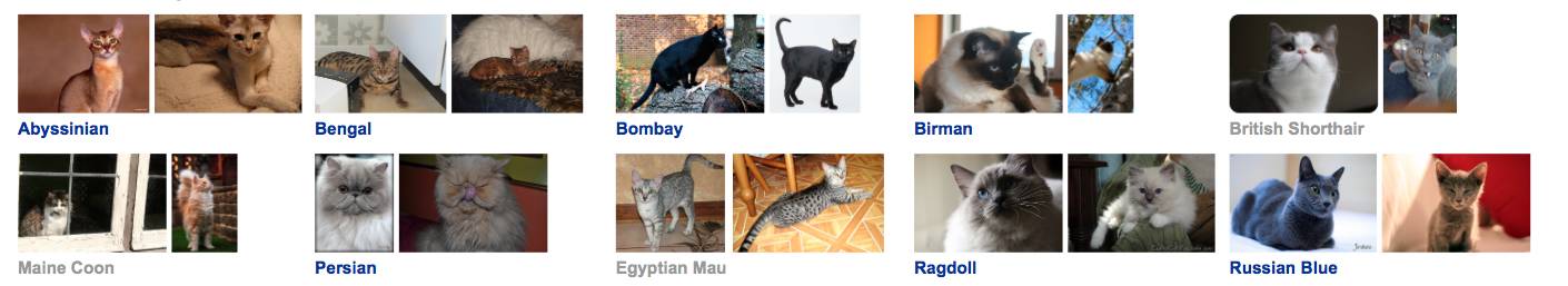
In this project, the categories we used are [Sphynx cat, Siamese cat, Ragdoll cat, Persian cat, Maine Coon, British Shorthair, Bombay cat, Burmese cat, Bengal cat, Abyssinian cat].
Therefore, we have a total of 2000 images in the dataset. Although the sizes of the images are different, we can resize them to a fixed size such as 64×64 or 128×128.
Preprocessing
In this project, we mainly use OpenCV for preprocessing the images, such as reading images into arrays or resizing them as needed.
A common method to improve image training results is to randomly deform, crop, or adjust the brightness of the training inputs. By using all possible variants of the same image, this method not only has the advantage of expanding the effective training data size but also helps the network to learn to handle all distortions that may occur in real life.
For specifics, please see: https://github.com/aleju/imgaug.
Evaluation
First method: The first part is to preprocess the dataset and use sklearn to apply KNN, SVM, and BP neural networks.
There are many parameters in the program that can be adjusted: in the image_to_feature_vector function, we set the image size to 128×128, and we previously tried using other sizes (such as 8×8, 64×64, 256×256) for training. We found that while larger image sizes yield better results, larger images also increase execution time and memory requirements. Therefore, we ultimately decided to use an image size of 128×128, as it is not too large while still ensuring accuracy.
In the extract_color_histogram function, we set the binary values for each channel to 32,32,32. In the previous function, we also tried 8, 8, 8 and 64, 64, 64. Although higher values can yield better results, they also require longer execution times, so we found 32,32,32 to be more appropriate.
For the dataset, we trained three types. The first type has 400 images and 2 labels in a sub-dataset. The second type has 1000 images and 5 labels in a sub-dataset. The last type has 1997 images and 10 labels in the full dataset. We parsed different datasets as parameters into the program.
In KNeighborsClassifier, we only changed the number of neighbors and stored the classification results of each dataset’s optimal K value. All other parameters were set to default.
In MLPClassifier, we set each hidden layer to have 50 neurons. We did test multiple hidden layers, but it seemed that there was no significant change in the final results. The maximum number of iterations was set to 1000, and to ensure that the model could converge, we tolerated a deviation of 1e-4. We also needed to set the L2 penalty’s alpha parameter to the default value, random state to 1, and the solver to ‘sgd’ with a learning rate of 0.1.
In SVC, the maximum number of iterations is set to 1000, and the class weight is set to ‘balanced’.
The runtime of our program is not too long, taking about 3 to 5 minutes for our three datasets.
Second method: Build CNN using TensorFlow
Using the entire large dataset would take a long time to compute the model’s gradients, so we update the weights using only small batches of images in each iteration of the optimizer, with a batch size typically being 32 or 64. The dataset is divided into a training set containing 1600 images, a validation set containing 400 images, and a test set containing 300 images.
This model also has many parameters that need to be adjusted.
The first is the learning rate. A good learning rate is small enough to allow the model to converge easily while being large enough to prevent the convergence from being too slow. So we chose 1 x 10^-4.
The second parameter that needs adjustment is the image size input into the network. We trained with both 64×64 and 128×128 image sizes, and the results showed that larger sizes lead to higher model accuracy, but at the cost of longer running times.
Then there is the number of layers and the shape of the neural network. However, in reality, there are too many parameters to adjust in this aspect, making it difficult to find an optimal value among all parameters.
Based on many resources online, we found that for building neural networks, parameter selection is largely based on existing experience.
Initially, we hoped to build a fairly complex neural network with the following parameters:
-
# Convolutional Layer 1. filter_size1 = 5 num_filters1 = 64
-
# Convolutional Layer 2. filter_size2 = 5 num_filters2 = 64
-
# Convolutional Layer 3. filter_size3 = 5 num_filters3 = 128
-
# Fully-connected layer 1. fc1_size = 256
-
# Fully-connected layer 2. fc1_size = 256
We used 3 convolutional layers and 2 fully connected layers, all with relatively complex structures.
However, our result was overfitting. For such a complex network, the training accuracy reached 100% after 1000 iterations, but the test accuracy was only 30%. At first, we were puzzled as to why the model was overfitting, and then we started adjusting parameters randomly, but the model’s performance improved. Luckily, a few days later, I happened to read an article by Google discussing deep learning: https://medium.com/@blaisea/physiognomys-new-clothes-f2d4b59fdd6a. The article pointed out that their project was problematic: “A technical issue is that if there are fewer than 2000 samples, it is insufficient to train and test a convolutional neural network like AlexNet without overfitting.” So I realized that our dataset was too small, and the network architecture was too complex, which led to overfitting.
Our dataset contains exactly 2000 images
Therefore, I began to reduce the number of layers in the neural network and the size of the kernels. I tried adjusting many parameters, and here are the parameters of the neural network architecture we ultimately used:
-
# Convolutional Layer 1. filter_size1 = 5 num_filters1 = 64
-
# Convolutional Layer 2. filter_size2 = 3 num_filters2 = 64
-
# Fully-connected layer 1. fc1_size = 128
-
# Number of neurons in fully-connected layer.
-
# Fully-connected layer 2. fc2_size = 128
-
# Number of neurons in fully-connected layer.
-
# Number of color channels for the images: 1 channel for gray-scale. num_channels = 3
We only used 2 small convolutional layers and 2 fully connected layers. The training results were not good, and overfitting occurred again after 4000 iterations, but the test accuracy was still 10% higher than the previous model.
We are still looking for solutions, but an obvious reason is that our dataset is indeed too small, and we do not have enough time to make further improvements.
As a final result, we achieved about 43% accuracy after 5000 iterations, which took an hour and a half. In fact, we were quite disappointed with this result, so we prepared to use another standard dataset, CIFAR-10.
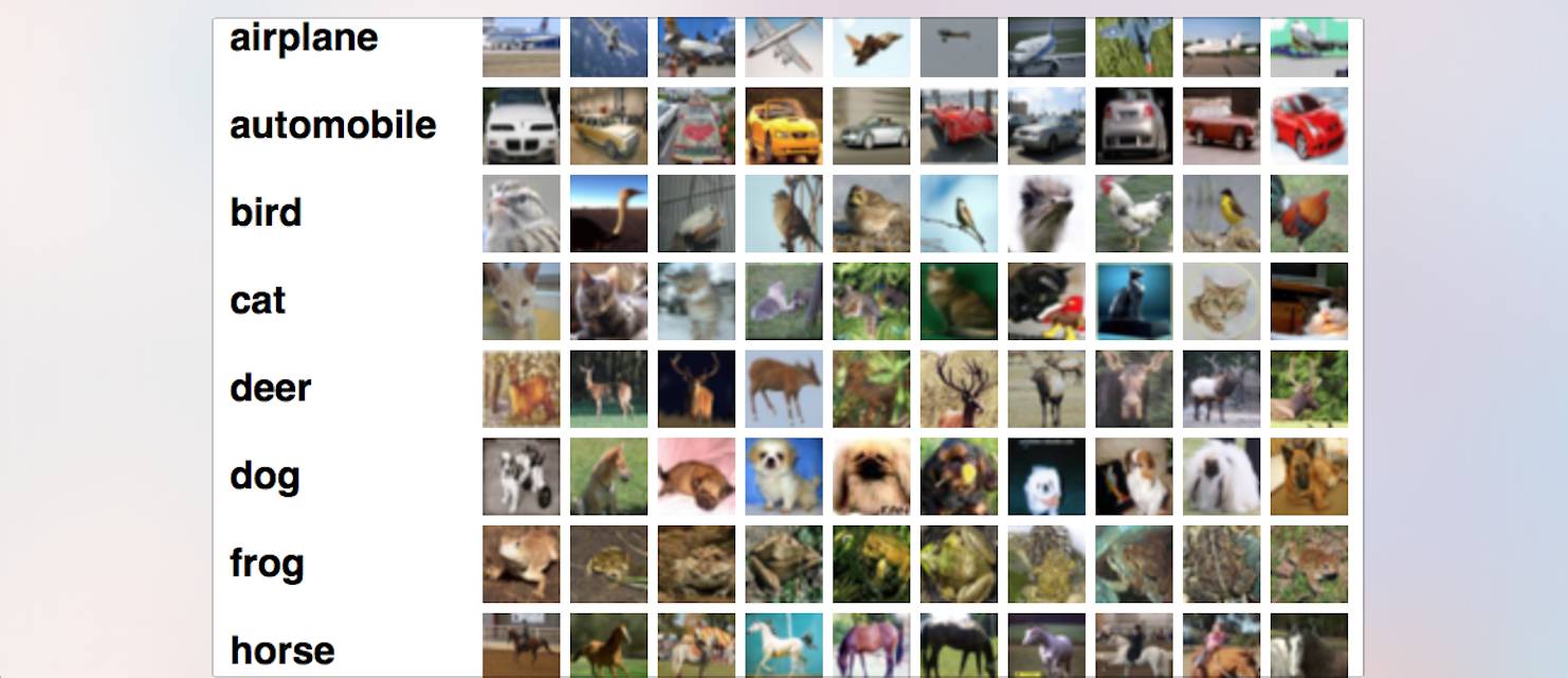
The CIFAR-10 dataset consists of 60,000 32×32 color images in 10 classes, with 6,000 images per class. This dataset contains 50,000 training images and 10,000 test images.
We used the same neural network architecture as above, and after 10 hours of training, we achieved 78% accuracy on the test set.
Third method: Retrain Inception V3. We randomly selected some images for training, while another batch of images was used for validation.
This model also has many parameters that need to be adjusted.
The first is the number of training steps, with the default value being 4000 steps. We can increase or decrease this based on the situation to quickly obtain an acceptable result.
Then there is the learning rate, which controls the magnitude of updates to the last layer during training. Intuitively, if the learning rate is small, it will take more time to learn, but ultimately it might converge to a better global accuracy. The training batch size controls how many images are checked in one training step, and since the learning rate is applied to each batch, if similar global effects can be achieved with a larger batch, we need to reduce it.
Because deep learning tasks typically require long running times, we do not want the model to perform poorly after training for several hours. Therefore, we need to frequently obtain reports on validation accuracy. This way we can also avoid overfitting. The dataset split involves allocating 80% of the images to the main training set, 10% of the images to a validation set that is frequently checked during training, and the remaining 10% of the images to the final test set to predict the classifier’s performance in the real world.
Results
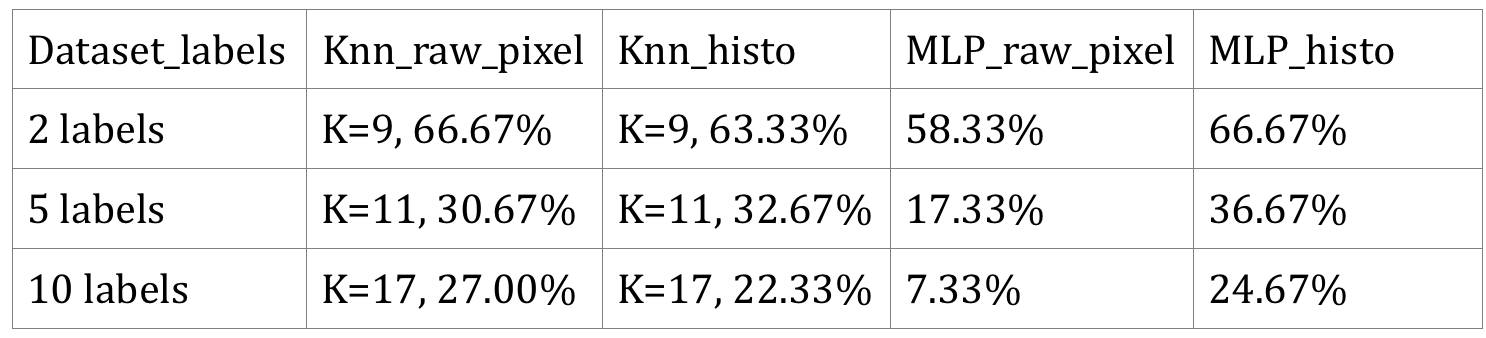
First category: Preprocess the dataset and implement KNN, SVM, and BP neural networks using sklearn.
The results are shown in the table below. Since the SVM results were very poor, even lower than random guessing, we will not present its results.
From the results, we see:
-
In k-NN, the accuracy of raw pixels and histograms is relatively equal. In the sub-dataset with 5 labels, the histogram accuracy is slightly higher than that of raw pixels; however, overall, the raw pixel results are better.
-
In the MLP classifier neural network, the accuracy of raw pixels is far lower than that of the histogram. For the entire dataset (10 labels), the accuracy of raw pixels is even lower than random guessing.
-
Both of these sklearn methods did not perform well, with the accuracy of correctly identifying classifications in the entire dataset (10 label dataset) being only about 24%. These results indicate that classification of images using sklearn is poor, and they do not perform well when classifying complex images with multiple categories. However, compared to random guessing, they do show some improvement, just not enough.
Based on the above results, we find that to improve accuracy, it is necessary to use some deep learning methods.
Second category: Build CNN using TensorFlow. As mentioned above, we cannot obtain good results due to overfitting.
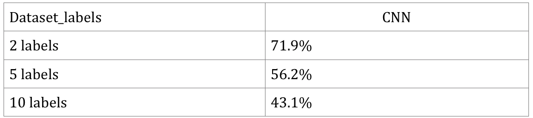
Normally, training takes half an hour; however, due to the results being overfitted, we think this runtime is not important. By comparing with the first category methods, we see that although CNN overfitted the training data, I still obtained better results.
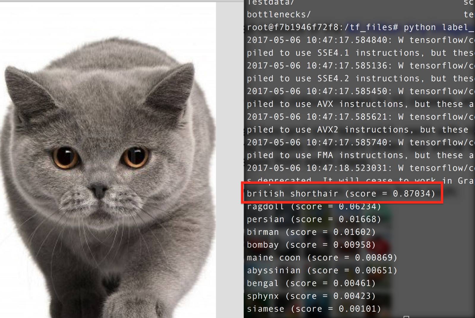
Third category: Retrain Inception V3
The entire training process took no more than 10 minutes. We achieved excellent results and truly witnessed the power of deep learning and transfer learning.
Demonstration:
Conclusion
Based on the above comparisons, we can see:
-
KNN, SVM, and BP neural networks are insufficient for certain specific image classification tasks.
-
Although we overfit in CNN, it is still better than those classroom methods.
-
Transfer learning is highly efficient and powerful for image classification problems. It is accurate and fast, can complete training in a short time—and does not require the help of a GPU. Even if you only have a very small dataset, it can achieve good results and reduces the probability of overfitting.
We have learned a lot from the image classification task, which is quite different from other classification tasks in class. The datasets are relatively large and dense, requiring very complex networks, and most methods rely on the computational power of GPUs.
Experience:
-
Crop or resize images to make them smaller
-
Randomly select a small batch in each iteration of training
-
Randomly select a small batch during validation on the validation set, frequently record validation scores during training
-
Image Augmentation can be used to process images, increasing the size of the dataset
-
For image classification tasks, we need a larger dataset than 200 x 10; the CIFAR-10 dataset contains 60,000 images.
-
More complex networks require larger datasets for training
-
Be cautious of overfitting
Note: The first method was implemented by Ji Tong: https://github.com/JI-tong 
References
1. CS231n Convolutional Neural Networks for Visual Recognition: http://cs231n.github.io/convolutional-networks/
2. TensorFlow Convolutional Neural Networks: https://www.tensorflow.org/tutorials/deep_cnn
3. How to Retrain Inception’s Final Layer for New Categories: https://www.tensorflow.org/tutorials/image_retraining
4. k-NN classifier for image classification: http://www.pyimagesearch.com/2016/08/08/k-nn-classifier-for-image-classification/
5. Image Augmentation for Deep Learning With Keras: http://machinelearningmastery.com/image-augmentation-deep-learning-keras/
6. Convolutional Neural Network TensorFlow Tutorial: https://github.com/Hvass-Labs/TensorFlow-Tutorials/blob/master/02_Convolutional_Neural_Network.ipynb
Click to read the original text, view the full guest lineup, and register to participate in Machine Heart GMIS 2017 ↓↓↓