Machine learning is an important branch of artificial intelligence, playing an increasingly significant role in areas such as data analysis, image recognition, and natural language processing in recent years. The basic concept of machine learning revolves around how to enable computers to learn and predict using data. R, as a powerful tool for statistical analysis and graphical representation, holds a place in the field of machine learning due to its rich packages and flexible data processing capabilities. Today we begin the first article on R language machine learning, focusing on data preparation and batch installation of packages.
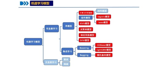
Machine learning is a discipline that studies how to enable computer systems to learn from data and improve performance. It achieves automatic processing and analysis of data by training models to identify patterns, predict trends, and make decisions.
Machine learning algorithms learn from large amounts of data, extracting useful features and building models to predict new data. These models can be continuously optimized to adapt to different types of data and tasks. Common machine learning algorithms include KNN, decision trees, random forests, Bayesian methods, etc.
First, we open Rstudio. You are probably already familiar with installing and loading individual packages:
rm(list=ls()) # Remove all variable data
install.packages() # Install package
library() # Load package
Then, to read and write Excel, we need to use the readxl and writexl packages:
# Read Excel data
install.packages(“readxl”)
library(readxl) # Load package
data <- read_excel(“path/example_data.xlsx”)
# Write Excel data export
install.packages(“writexl”)
library(writexl) # Load package
write_xlsx(data.all, “path/summary.xlsx”)
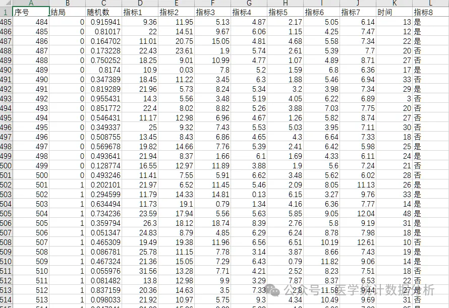
Today, we will use a sample data set consisting of 1000 cases. We will read it into Rstudio for processing using readxl.
We can
# Define the list of packages needed for machine learning, check if each package is already installed, and if not, install and load it
packages<-c(“readxl”,”ggplot2″,”caret”,”lattice”,”gmodels”,
“glmnet”,”Matrix”,”pROC”,”Hmisc”,”rms”,
“tidyverse”,”Boruta”,”car”,”carData”,
“rmda”,”dplyr”,”rpart”,”rattle”,”tibble”,”bitops”,
“probably”,”tidymodels”,”fastshap”,
“shapviz”,”e1071″)
for(pkg in packages) {
if (!require(pkg, quietly = TRUE)) {
install.packages(pkg, dependencies = TRUE)
library(pkg, character.only = TRUE)
}
}
# Use library() function to load multiple packages at once
lapply(packages,library,character.only = TRUE)
Alternatively, we can
# Directly define and batch install packages
packages<-c(“readxl”,”ggplot2″,”caret”,
“lattice”,”gmodels”,”glmnet”,”Matrix”,”pROC”,
“Hmisc”,”rms”,”tidyverse”,”Boruta”,”car”,
“carData”,”rmda”,”dplyr”,”rpart”,”rattle”,”tibble”,
“bitops”,”probably”,”tidymodels”,”fastshap”,
“shapviz”,”e1071″)
install.packages(c(“readxl”,”ggplot2″,”caret”,
“lattice”,”gmodels”,”glmnet”,”Matrix”,”pROC”,
“Hmisc”,”rms”,”tidyverse”,”Boruta”,”car”,”carData”,
“rmda”,”dplyr”,”rpart”,”rattle”,”tibble”,”bitops”, “probably”,”tidymodels”,”fastshap”,
“shapviz”,”e1071″))
install.packages(packages)
# Use library() function to load multiple packages at once
lapply(packages,library,character.only = TRUE)
Furthermore, we can perform simple analysis:
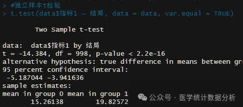
# Independent samples t-test
t.test(data$indicator1 ~ outcome, data = data, var.equal = TRUE)
t.test(data$indicator2 ~ outcome, data = data, var.equal = TRUE)
t.test(data$indicator3 ~ outcome, data = data, var.equal = TRUE)
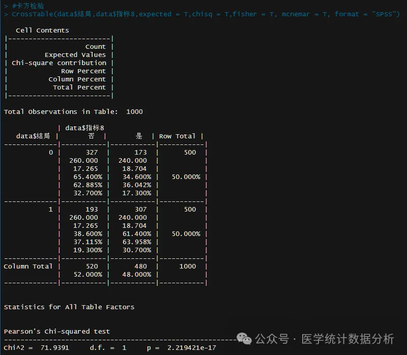
# Chi-square test
CrossTable(data$outcome,data$indicator8,expected = T,chisq = T,fisher = T, mcnemar = T, format = “SPSS”)
# Logistic regression
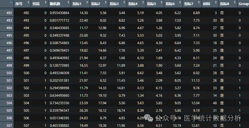
data$Group<-as.factor(data$outcome)
model1 <- glm(Group ~ indicator1, data = data, family = “binomial”)
summary(model1)
model2 <- glm(Group ~ indicator1+indicator2, data = data, family = “binomial”)
summary(model2)
model3 <- glm(Group ~ indicator1+indicator2+indicator3, data = data, family = “binomial”)
summary(model3)

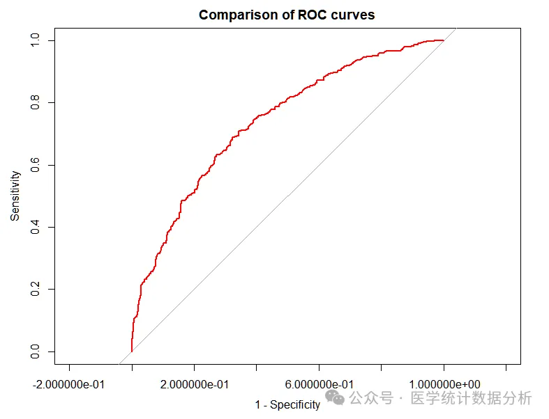
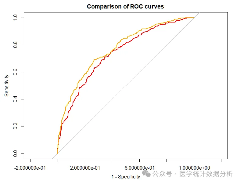
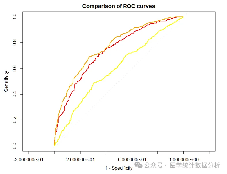
# ROC curve
roc1 <- roc(data$outcome,data$indicator1);roc1
roc2 <- roc(data$outcome,data$indicator2);roc2
roc3 <- roc(data$outcome,data$indicator3);roc3
plot(roc1,
max.auc.polygon=FALSE, # Fill the entire image
smooth=F, # Draw unsmoothed curve
main=”Comparison of ROC curves”, # Add title
col=”red”, # Curve color
legacy.axes=TRUE) # Make the x-axis range from 0 to 1, representing 1-specificity
plot.roc(roc2,
add=T, # Add curve
col=”orange”, # Curve color is red
smooth = F) # Draw unsmoothed curve
plot.roc(roc3,
add=T, # Add curve
col=”yellow”, # Curve color is red
smooth = F) # Draw unsmoothed curve
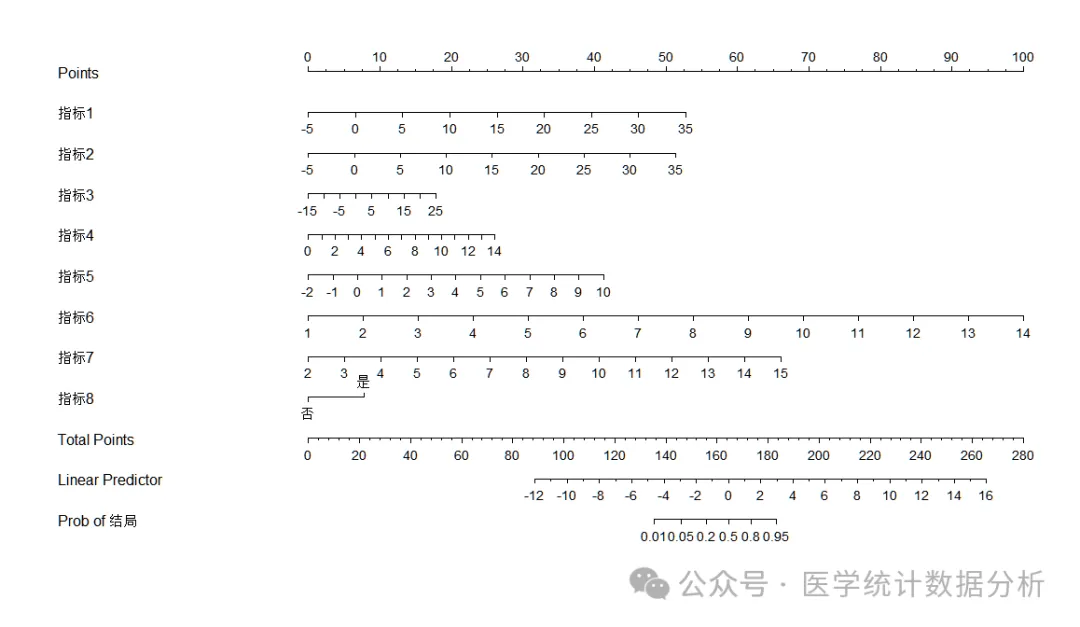
# Nomogram
dd<-datadist(data)
options(datadist=”dd”)
data$Group<-as.factor(data$outcome)
f_lrm<-lrm(Group~indicator1+indicator2+indicator3+indicator4+indicator5+indicator6+indicator7+indicator8,data=data)
summary(f_lrm)
par(mgp=c(1.6,0.6,0),mar=c(5,5,3,1))
nomogram <- nomogram(f_lrm,fun=function(x)1/(1+exp(-x)),
fun.at=c(0.01,0.05,0.2,0.5,0.8,0.95,1),
funlabel =”Prob of outcome”,
conf.int = F,
abbrev = F )
plot(nomogram)
The training set and test set are commonly used data partitioning methods in deep learning technology. They automatically divide the data into training and test sets for the evaluation of model development.
The training set is a group of data prepared for training the model, which is usually labeled by humans to indicate they possess specific attributes. Generally, to train an effective model, the sample size of the training set should be large enough and should have sufficient diversity to represent all possible scenarios in their dataset.
The test set is a group of samples used to test the trained model, verifying the accuracy and correctness of the trained model. It essentially consists of unknown data samples used to evaluate model performance without the bias of training set sampling, providing a more reliable assessment of the model’s performance.
So how do we partition the test and training sets?
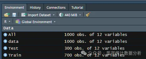
# Stratified sampling to partition training and test sets
set.seed(123)
train <- sample(1:nrow(data),nrow(data)*7/10) # Take 70% for training set, remaining 30% for test set
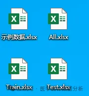
# Data reading, splitting, and combining
Train <- data[train,] # Define training set data
Test <- data[-train,] # Define test set data
All <- rbind(Train, Test) # Combine split data
# Write Excel data export
install.packages(“writexl”)
library(writexl) # Load package
write_xlsx(Train, “C:/Users/L/Desktop/Train.xlsx”)
write_xlsx(Test, “C:/Users/L/Desktop/Test.xlsx”)
write_xlsx(All, “C:/Users/L/Desktop/All.xlsx”)