

Author: louwill
Although deep learning is currently very popular, Boosting algorithms represented by XGBoost, LightGBM, and CatBoost still have a wide range of applications. Leaving aside the applications of deep learning suitable for unstructured data such as images, text, speech, and video, Boosting algorithms remain the first choice for structured data with fewer training samples. This article first briefly explains the connections and differences among the three Boosting algorithms mentioned above and compares them using a practical data case. Then, it introduces common hyperparameter tuning methods for Boosting algorithms, including random search, grid search, and Bayesian optimization, along with corresponding code examples.
Comparison of the Three Boosting Algorithms
Firstly, XGBoost, LightGBM, and CatBoost are currently classic state-of-the-art (SOTA) Boosting algorithms, all of which can be classified into the gradient boosting decision tree algorithm series. All three models are based on decision trees in an ensemble learning framework, where XGBoost is an improvement over the original GBDT algorithm, while LightGBM and CatBoost have further optimized it, each with its own advantages in accuracy and speed.
So what are the major differences among these three Boosting algorithms? There are mainly two aspects. The first is that the tree construction methods of the three models are different: XGBoost uses a level-wise growth strategy for decision trees, LightGBM uses a leaf-wise growth strategy, while CatBoost employs a symmetric tree structure, where the decision trees are complete binary trees. The second significant difference lies in the handling of categorical features. XGBoost does not have the capability to automatically handle categorical features; for categorical features in the data, we need to manually transform them into numerical values before inputting them into the model. In LightGBM, categorical feature names need to be specified, and the algorithm can handle them automatically; CatBoost is well-known for handling categorical features efficiently through methods such as target variable statistics and feature encoding.
Next, we will use the Kaggle 2015 flight delay dataset as an example and conduct experiments using XGBoost, LightGBM, and CatBoost models. Figure 1 provides an overview of the flights dataset.

Figure 2 Flights Dataset
The complete dataset contains over 5 million flight records with 31 features. For demonstration purposes, we sampled 1% of the original dataset and selected 11 features. After preprocessing, we reconstructed the training dataset, aiming to build a binary classification model to predict whether flights are delayed. The data reading and simple preprocessing process is shown in Code 1.
Code 1 Data Processing
# Import pandas and sklearn data splitting module
import pandas as pd
from sklearn.model_selection import train_test_split
# Read flights dataset
flights = pd.read_csv('flights.csv')
# Sample 1% of the dataset
flights = flights.sample(frac=0.01, random_state=10)
# Feature sampling, select specified 11 features
flights = flights[["MONTH", "DAY", "DAY_OF_WEEK", "AIRLINE",
"FLIGHT_NUMBER","DESTINATION_AIRPORT", "ORIGIN_AIRPORT","AIR_TIME",
"DEPARTURE_TIME", "DISTANCE", "ARRIVAL_DELAY"]]
# Discretize labels, only delays over 10 minutes count as delayed
flights["ARRIVAL_DELAY"] = (flights["ARRIVAL_DELAY"]>10)*1
# Categorical features
cat_cols = ["AIRLINE", "FLIGHT_NUMBER", "DESTINATION_AIRPORT",
"ORIGIN_AIRPORT"]
# Categorical feature encoding
for item in cat_cols:
      flights[item] = flights[item].astype("category").cat.codes +1
  # Split dataset
X_train, X_test, y_train, y_test = train_test_split(
      flights.drop(["ARRIVAL_DELAY"], axis=1),
      flights["ARRIVAL_DELAY"],
      random_state=10, test_size=0.3)
# Print sizes of the split datasets
print(X_train.shape, y_train.shape, X_test.shape, y_test.shape)
Output:
(39956, 10) (39956,) (17125, 10) (17125,)In Code 1, we first read the original flights dataset. Because the original dataset is too large, we sample 1% of it and select 11 features to create a dataset with 57,081 flight records and 11 features. We then perform simple preprocessing on the sampled dataset, discretizing the training labels into binary values, where delays greater than 10 minutes are converted to 1 (delayed), and delays less than 10 minutes are converted to 0 (not delayed). We also encode categorical features such as “Airline”, “Flight Number”, “Destination Airport”, and “Origin Airport”. Finally, we split the dataset, resulting in 39,956 training samples and 17,125 testing samples.
XGBoost
Next, we will test the performance of the three models on this dataset, starting with XGBoost, as shown in Code 2.
Code 2 XGBoost
# Import xgboost module
import xgboost as xgb
# Import model evaluation AUC function
from sklearn.metrics import roc_auc_score
# Set model hyperparameters
params = {
    'booster': 'gbtree',
    'objective': 'binary:logistic',
    'gamma': 0.1,
    'max_depth': 8,
    'lambda': 2,
    'subsample': 0.7,
    'colsample_bytree': 0.7,
    'min_child_weight': 3,
    'eta': 0.001,
    'seed': 1000,
    'nthread': 4,
}
# Wrap xgboost dataset
dtrain = xgb.DMatrix(X_train, y_train)
# Number of training rounds, i.e., number of trees
num_rounds = 500
# Model training
model_xgb = xgb.train(params, dtrain, num_rounds)
# Predict on the test set
dtest = xgb.DMatrix(X_test)
y_pred = model_xgb.predict(dtest)
print('AUC of testset based on XGBoost: ', roc_auc_score(y_test, y_pred))
Output:
AUC of testset based on XGBoost: 0.6845368959487046In Code 2, we tested XGBoost‘s performance on the flights dataset by importing relevant modules and setting model hyperparameters. We fit the XGBoost model based on the training set, and finally used the trained model for predictions on the test set, obtaining an AUC of 0.6845.
LightGBM
The testing process of LightGBM on the flights dataset is shown in Code 3.
Code 3 LightGBM
# Import lightgbm module
import lightgbm as lgb
dtrain = lgb.Dataset(X_train, label=y_train)
params = {
"max_depth": 5,
"learning_rate" : 0.05,
"num_leaves": 500,
"n_estimators": 300
}

# Specify categorical features
cate_features_name = ["MONTH","DAY","DAY_OF_WEEK","AIRLINE",
"DESTINATION_AIRPORT", "ORIGIN_AIRPORT"]
  # Fit lightgbm model
model_lgb = lgb.train(params, dtrain,
categorical_feature = cate_features_name)
  # Predict on the test set
y_pred = model_lgb.predict(X_test)
print('AUC of testset based on LightGBM: ', roc_auc_score(y_test, y_pred))
Output:
AUC of testset based on LightGBM: 0.6873707383550387In Code 3, we tested LightGBM‘s performance on the flights dataset. By importing relevant modules and setting model hyperparameters, we fit the LightGBM model based on the training set and used the trained model for predictions on the test set, obtaining an AUC of 0.6873, which is similar to that of XGBoost.
CatBoost
The testing process of CatBoost on the flights dataset is shown in Code 4.
Code 4 CatBoost
# Import catboost module
import catboost as cb
# Categorical feature indices
cat_features_index = [0,1,2,3,4,5,6]
# Create catboost model instance
model_cb = cb.CatBoostClassifier(eval_metric="AUC",
  one_hot_max_size=50, depth=6, iterations=300, l2_leaf_reg=1,
  learning_rate=0.1)
# Fit catboost model
model_cb.fit(X_train, y_train, cat_features=cat_features_index)
# Predict on the test set
y_pred = model_cb.predict(X_test)
print('AUC of testset based on CatBoost: ', roc_auc_score(y_test, y_pred))
Output:
AUC of testset based on CatBoost: 0.5463773041667715In Code 4, we tested CatBoost‘s performance on the flights dataset. By importing relevant modules and setting model hyperparameters, we fit the CatBoost model based on the training set and used the trained model for predictions on the test set, obtaining an AUC of 0.54, which is significantly lower than XGBoost and LightGBM. Table 1 shows the comprehensive comparison results of the three models on the flights dataset.
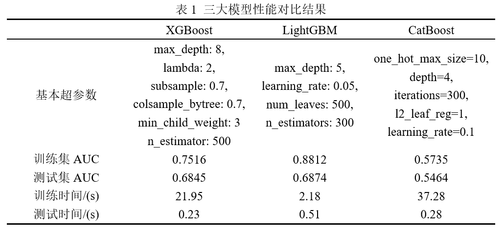
From the comprehensive comparison results in Table 1, LightGBM outperforms both XGBoost and CatBoost in terms of both accuracy and speed. Of course, we only compared the three models directly on the dataset without further feature engineering or hyperparameter tuning, so the results in Table 1 can be further optimized.
Common Hyperparameter Tuning Methods
In machine learning models, there are many parameters that need to be set manually in advance, such as the batch size for training neural networks and tree-related parameters for ensemble learning models like XGBoost. We refer to these parameters that are not derived from model training as hyperparameters. The process of manually adjusting hyperparameters is what we commonly refer to as hyperparameter tuning. Common tuning methods in machine learning include grid search, random search, and Bayesian optimization.
Grid Search
Grid search is a commonly used hyperparameter tuning method, often used to optimize three or fewer hyperparameters. Essentially, it is an exhaustive search method. For each hyperparameter, the user selects a small finite set to explore. Then, the Cartesian product of these hyperparameters yields several sets of hyperparameters. Grid search trains the model using each set of hyperparameters and selects the one with the smallest validation set error as the best hyperparameters.
For example, if we have three hyperparameters to optimize, a, b, and c, with candidate values {1,2}, {3,4}, and {5,6}, respectively, the possible combinations of parameter values form an 8-point 3-dimensional grid as follows: {(1,3,5),(1,3,6),(1,4,5),(1,4,6),(2,3,5),(2,3,6),(2,4,5),(2,4,6)}. Grid search traverses these 8 possible parameter combinations for training and validation to ultimately find the optimal hyperparameters.
In Sklearn, grid search tuning can be implemented using the GridSearchCV module in the model_selection package. We will also use the aforementioned flights dataset to demonstrate an example of grid search with XGBoost.
Code 5 Grid Search
### Example of GridSearch search based on XGBoost
# Import GridSearch module
from sklearn.model_selection import GridSearchCV
# Create xgb classification model instance
model = xgb.XGBClassifier()
# List of parameters to search
param_lst = {"max_depth": [3,5,7],
              "min_child_weight" : [1,3,6],
              "n_estimators": [100,200,300],
              "learning_rate": [0.01, 0.05, 0.1]
             }
# Create grid search
grid_search = GridSearchCV(model, param_grid=param_lst, cv=3,
                                   verbose=10, n_jobs=-1)
# Execute search based on flights dataset
grid_search.fit(X_train, y_train)
# Output search results
print(grid_search.best_estimator_)
Output:
XGBClassifier(max_depth=5, min_child_weight=6, n_estimators=300)Code 5 provides an example of grid search based on XGBoost. We first create an XGBoost classification model instance, then specify the parameters and their ranges to search, create a grid search object based on GridSearch, fit the training data, and output the grid search parameter results. We can see that when the maximum tree depth is 5, the minimum child weight is 6, and the number of trees is 300, the model achieves relatively optimal performance.
Random Search
Random search, as the name suggests, involves randomly searching for the optimal hyperparameters within a specified range or distribution. Compared to grid search, not every hyperparameter within the given distribution will be attempted; instead, a fixed number of parameters will be sampled from the given distribution, and only these sampled hyperparameters will be tested. Random search can sometimes be a more efficient tuning method than grid search. In Sklearn, random search tuning can be implemented using the RandomizedSearchCV method in the model_selection package. An example of random search tuning based on XGBoost is shown in Code 6.
Code 6 Random Search
### Example of RandomizedSearch search based on XGBoost
# Import GridSearch module
from sklearn.model_selection import GridSearchCV
# Create xgb classification model instance
model = xgb.XGBClassifier()
# List of parameters to search
param_lst = {"max_depth": [3,5,7],
              "min_child_weight" : [1,3,6],
              "n_estimators": [100,200,300],
              "learning_rate": [0.01, 0.05, 0.1]
             }
# Create grid search
grid_search = GridSearchCV(model, param_grid=param_lst, cv=3,
                                   verbose=10, n_jobs=-1)
# Execute search based on flights dataset
grid_search.fit(X_train, y_train)
# Output search results
print(grid_search.best_estimator_)
Output:
XGBClassifier(max_depth=5, min_child_weight=6, n_estimators=300)Code 6 provides an example of random search, which is similar to grid search in structure. We can see that the random search results suggest that the number of trees should be 300, the minimum child weight should be 6, the maximum depth should be 5, and the learning rate should be 0.1 for optimal model performance.
Bayesian Optimization
In addition to the aforementioned tuning methods, this section introduces a third method that may be the best one, namely Bayesian optimization. Bayesian optimization is a parameter optimization method based on Gaussian processes and Bayesian theorem, which has been widely used for hyperparameter tuning in machine learning models in recent years. Here, we will not delve into the mathematical principles of Gaussian processes and Bayesian optimization, but will showcase the basic usage and tuning example of Bayesian optimization.
Bayesian optimization, like other optimization methods, aims to find the parameter values that maximize the objective function. As a sequential optimization problem, Bayesian optimization requires selecting the best observation value in each iteration, which is the key issue in Bayesian optimization. This key issue is perfectly solved by the aforementioned Gaussian processes. Due to space limitations, we will not elaborate on the mathematical principles of Bayesian optimization, including concepts such as Gaussian processes, acquisition functions, Upper Confidence Bound (UCB), and Expectation Improvements (EI). Bayesian optimization can be implemented using the existing third-party library BayesianOptimization. The usage example is shown in Code 7.
Code 7 Bayesian Optimization
### Example of BayesianOptimization search based on XGBoost
# Import xgboost module
import xgboost as xgb
# Import Bayesian optimization module
from bayes_opt import BayesianOptimization
# Define objective optimization function
def xgb_evaluate(min_child_weight,
                 colsample_bytree,
                 max_depth,
                 subsample,
                 gamma,
                 alpha):
    # Specify hyperparameters to optimize
    params['min_child_weight'] = int(min_child_weight)
    params['cosample_bytree'] = max(min(colsample_bytree, 1), 0)
    params['max_depth'] = int(max_depth)
    params['subsample'] = max(min(subsample, 1), 0)
    params['gamma'] = max(gamma, 0)
    params['alpha'] = max(alpha, 0)
    # Define xgb cross-validation results
    cv_result = xgb.cv(params, dtrain, num_boost_round=num_rounds, nfold=5,
                   seed=random_state,
                   callbacks=[xgb.callback.early_stop(50)])
    return cv_result['test-auc-mean'].values[-1]

# Define relevant parameters
num_rounds = 3000
random_state = 2021
num_iter = 25
init_points = 5
params = {
    'eta': 0.1,
    'silent': 1,
    'eval_metric': 'auc',
    'verbose_eval': True,
    'seed': random_state
}
# Create Bayesian optimization instance
# and set parameter search range
xgbBO = BayesianOptimization(xgb_evaluate,
                             {'min_child_weight': (1, 20),
                               'colsample_bytree': (0.1, 1),
                               'max_depth': (5, 15),
                               'subsample': (0.5, 1),
                               'gamma': (0, 10),
                               'alpha': (0, 10),
                                })
# Execute tuning process
xgbBO.maximize(init_points=init_points, n_iter=num_iter)
Code 7 provides an example of Bayesian optimization based on XGBoost. Before executing Bayesian optimization, we need to define an objective function based on XGBoost‘s cross-validation xgb.cv to optimize, obtaining xgb.cv cross-validation results and using the test set AUC as the accuracy metric for optimization. Finally, we pass the defined objective optimization function and hyperparameter search range into the Bayesian optimization function BayesianOptimization, specifying the number of initialization points and iterations to execute Bayesian optimization.
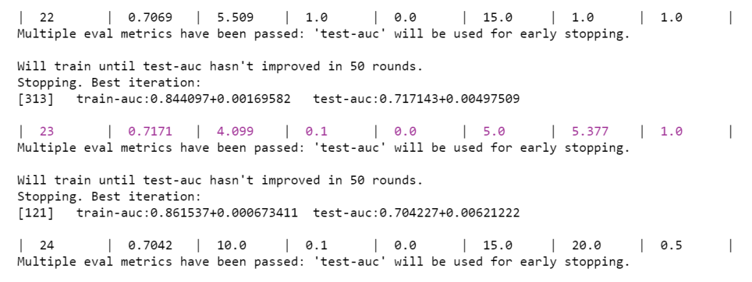
Figure 2 Bayesian Optimization Results
Part of the optimization process is shown in Figure 2, where we can see that Bayesian optimization reached its optimum at the 23rd iteration, with the parameters set as alpha = 4.099, column sampling ratio = 0.1, gamma = 0, maximum tree depth = 5, minimum child weight = 5.377, and subsampling ratio = 1.0, achieving an optimal test set AUC of 0.72.
Conclusion
This chapter provides a simple comprehensive comparison based on the previous chapters on ensemble learning and presents commonly used hyperparameter tuning methods and examples. We performed a performance comparison in terms of accuracy and speed among the three commonly used Boosting ensemble learning models: XGBoost, LightGBM, and CatBoost using a specific data instance. However, due to specific datasets and tuning differences, the comparison results are only for demonstration purposes and do not genuinely represent that the LightGBM model is always superior to the CatBoost model.
The three commonly used hyperparameter tuning methods are grid search, random search, and Bayesian optimization. This chapter also provides examples of using these three hyperparameter tuning methods based on the same dataset, but due to space limitations, we did not delve deeply into the mathematical principles of each method.
I am Dong Ge, and I am currently creating a series of original topics 👉「100 Cool Operations of Pandas」. Feel free to subscribe. After subscribing, updates will be pushed to your subscription account in real-time, so you won’t miss any articles.
Finally, I would like to share with you 100 Python E-books, which include Python programming tips, data analysis, web scraping, web development, machine learning, and deep learning.
This is now shared for free. Readers who need them can download and learn. Just reply with the keyword: Python in the public account GitHuboy.