BP Neural Network Algorithm and Practice

(Click the public account above to follow quickly)

Source: CodeMeals

cnblogs.com/fengfenggirl/p/bp_network.html

If you have good articles to submit, please click → here for details

Neural networks were once very popular, went through a period of decline, and are now gaining popularity again due to deep learning. There are many types of neural networks: feedforward networks, backpropagation networks, recurrent neural networks, convolutional neural networks, etc. This article introduces the basic backpropagation neural network (BP), focusing on the basic algorithm process and some of my experiences in training BP neural networks.

Structure of BP Neural Network

A neural network simulates the functioning of the nerve units in the human brain but simplifies it greatly. The neural network consists of many layers, each composed of many units. The first layer is called the input layer, the last layer is called the output layer, and the layers in between are called hidden layers. In a BP neural network, only adjacent layers are connected, and each layer, except for the output layer, has a bias node:

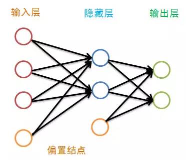
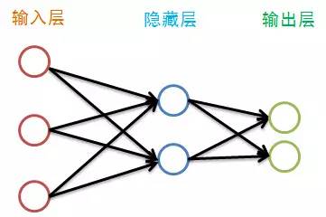
Although the hidden layer in the figure shows only one layer, there is no limit to the number of layers. Traditional neural network learning experience suggests that one layer is sufficient, while recent deep learning does not agree. The bias node is used to describe features not present in the training data, producing different biases for each node in the next layer based on the weights. Therefore, we can consider the bias as an attribute of each node (except for the input layer). We omit the bias nodes in the figure:

Before describing the training of the BP neural network, let’s first look at the attributes of each layer in the neural network:

1. Each neural unit has a certain amount of energy, defined as the output value Oj of node j;

2. The connection between adjacent layer nodes has a weight Wij, which is valued between [-1,1];

3. Each node in every layer, except for the input layer, has an input value equal to the sum of the energies transmitted from all nodes in the previous layer multiplied by their weights, plus the bias;

4. Each layer, except for the input layer, has a bias value ranging from [0,1];

5. The output value of each node, except for the input layer, is a nonlinear transformation of its input value;

6. We consider the input layer has no input values, and its output values are the attributes of the training data. For instance, for a record X=< (1,2,3), class 1 >, the output values of the three nodes in the input layer would be 1, 2, and 3. Therefore, the number of nodes in the input layer generally equals the number of attributes in the training data.

Training a BP neural network essentially involves adjusting the two parameters of the network: weights and biases. The training process of the BP neural network consists of two parts:

1. Feedforward transmission, where output values are passed layer by layer;

2. Backward feedback, where weights and biases are adjusted layer by layer;

Let’s first look at the feedforward transmission.

Feedforward Transmission

Before training the network, we need to randomly initialize the weights and biases, taking a random real number for each weight in the range of [-1,1] and a random real number for each bias in the range of [0,1], and then we begin the feedforward transmission.

The training of the neural network is completed through multiple iterations, each using all records from the training set, and each training session uses only one record. An abstract description is as follows:

while the termination condition is not met:

for record: dataset:

trainModel(record)

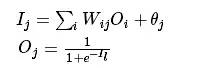
First, we set the output values of the input layer. Assuming the number of attributes is 100, we set the number of neural units in the input layer to 100, with each node Ni in the input layer corresponding to the attribute value xi of record dimension i. The operation for the input layer is that simple; the subsequent layers are a bit more complex. Each node’s input value in other layers (except the input layer) is the sum of the input values from the previous layer weighted and added to the bias, and the output value of each node is the transformation of its input value.

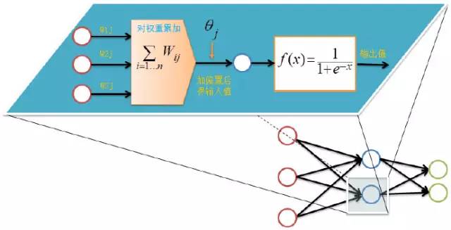
The calculation process for the output layer during feedforward transmission is as follows:

For every node in the hidden and output layers, the output values are calculated as shown in the above diagram, completing the feedforward process, followed by backward feedback.

Backward Feedback

Backward feedback starts from the last layer, the output layer. The purpose of training the neural network for classification is often to hope that the output of the last layer can describe the category of the data record. For a binary classification problem, we often use two neural units as the output layer. If the output value of the first neural unit in the output layer is greater than that of the second, we consider this data record belongs to the first category; otherwise, it belongs to the second category.

Remember that when we first performed feedforward, the entire network’s weights and biases were randomly assigned, so the network’s output could not describe the category of the record. Therefore, we need to adjust the network’s parameters, namely the weights and biases, based on the difference between the output value of the output layer and the category. The goal of neural network optimization is to minimize this difference. For the output layer:

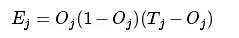
Where Ej represents the error value of the j-th node, Oj represents the output value of the j-th node, and Tj records the output value. For a binary classification problem, we use 01 to indicate category 1 and 10 to indicate category 2. If a record belongs to category 1, then T1=0 and T2=1.

The hidden layers do not directly interact with the data record’s category but accumulate errors from all nodes in the next layer weighted. The calculation formula is as follows:

Where Wjk represents the weight from the j-th node of the current layer to the k-th node of the next layer, and Ek represents the error rate of the k-th node in the next layer.

After calculating the error rate, we can update the weights and biases using the error rate. First, let’s look at updating the weights:

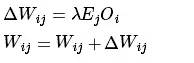
Where λ represents the learning rate, which takes values from 0 to 1. A larger learning rate leads to faster convergence but risks falling into local optima, while a smaller learning rate converges more slowly but approaches the global optimum step by step.

After updating the weights, there is one last parameter to update, which is the bias:

At this point, we have completed one training process of the neural network. By continuously using all data records for training, we obtain a classification model. The iterations cannot go on indefinitely; there must be a termination condition.

Training Termination Conditions

Each round of training uses all records from the dataset, but when to stop? The termination conditions are as follows:

1. Set a maximum number of iterations, for example, stop training after iterating through the dataset 100 times.

2. Calculate the prediction accuracy of the training set on the network and stop training once a certain threshold is reached.

Using BP Neural Network for Classification

I wrote a BP neural network myself and tested it on the handwritten digit recognition dataset MINIST. The MINIST dataset has 12,000 training images and 20,000 test images, with each image being a 28*28 grayscale image. I processed the images into binary format. The parameters of the neural network are set as follows:

1. Input layer set to 28*28=784 input units;

2. Output layer set to 10, corresponding to 10 digit categories;

3. Learning rate set to 0.05;

After about 50 iterations, I achieved a 99% accuracy on the training set, and the accuracy on the test set was 90.03%. The potential for improvement with a pure BP neural network is limited, but someone on Kaggle has achieved a 99.3% accuracy on the test set using convolutional neural networks. The code was written in C++ last year and has a strong JAVA flavor; its value is not high, but the comments are quite detailed. You can check it out here. Recently, I wrote a multi-threaded BP neural network in Java, but it’s not convenient to share yet. If the project fails, I’ll put it up later.

Some Experiences in Training BP Neural Networks

Here are some of my experiences in training neural networks:

1. The learning rate should not be set too high, generally less than 0.1. I initially set it to 0.85, and the accuracy did not improve, clearly falling into a local optimum;

2. Input data should be normalized. Initially, I tested with grayscale values from 0-255, but the results were poor. After converting to binary 01, the improvement was significant;

3. Data records should be randomly distributed; do not sort the dataset by records. For example, if the dataset has 10 categories and we sort it by category, training the neural network record by record will cause the model to only remember the most recently trained category while forgetting the earlier ones;

4. For multi-class problems, such as Chinese character recognition, there are more than 7,000 commonly used characters. If we set the output layer to 7,000 nodes, the computation will be enormous, and the parameters will be too many to converge easily. In this case, we should encode the categories, as 7,000 Chinese characters can be represented with just 13 binary bits. Therefore, we only need to set 13 nodes for the output.

References:

Jiawei Han. “Data Mining Concepts and Techniques”

If you find this article helpful, please share it with more people

Follow “Algorithm Enthusiasts” to improve your programming skills