Selected from GitHub
Author: Jay Alammar
Contributors: Wang Zijia, Geek AI
If you are a natural language processing practitioner, you must have heard of the recently popular BERT model.This article is a detailed tutorial on using a simplified version of the BERT model—DisTillBERT to complete the sentiment classification task of sentences, making it an invaluable quick start guide for BERT.
In recent years, machine learning models for processing language have made tremendous progress.These advancements have moved out of the laboratory and begun to empower some advanced digital products.The BERT model, which has recently become a major force behind Google Search, is a good example.Google believes this advancement (or the progress of applying natural language understanding technology in search) represents “the biggest leap in the past five years and one of the biggest leaps in the history of search.”
This article is a simple tutorial that introduces how to classify sentences using different BERT models.The examples in this article are straightforward and sufficient to illustrate the key concepts involved in using BERT.
In addition to this blog post, I have also prepared a corresponding notebook code, the link is as follows:
https://github.com/jalammar/jalammar.github.io/blob/master/notebooks/bert/A_Visual_Notebook_to_Using_BERT_for_the_First_Time.ipynb.
You can also run this code in Colab:
https://colab.research.google.com/github/jalammar/jalammar.github.io/blob/master/notebooks/bert/A_Visual_Notebook_to_Using_BERT_for_the_First_Time.ipynb
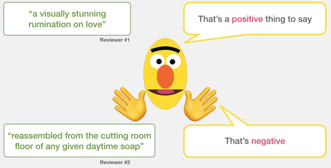
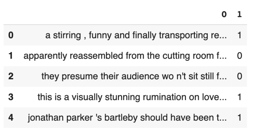
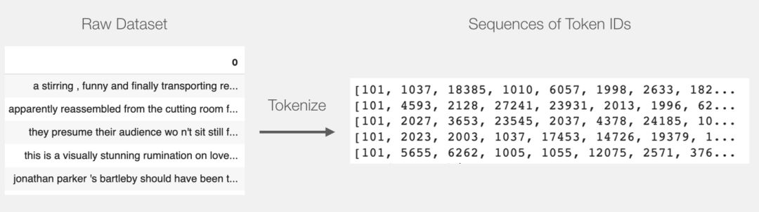
The dataset used in this example is “SST2”, which collects sentences from movie reviews, each labeled with positive reviews marked as 1 and negative reviews marked as 0.
| sentence |
label |
| a stirring , funny and finally transporting re imagining of beauty and the beast and 1930s horror films |
1 |
| apparently reassembled from the cutting room floor of any given daytime soap |
0 |
| they presume their audience won’t sit still for a sociology lesson |
0 |
| this is a visually stunning rumination on love , memory , history and the war between art and commerce |
1 |
| jonathan parker ‘s bartleby should have been the be all end all of the modern office anomie films |
1 |
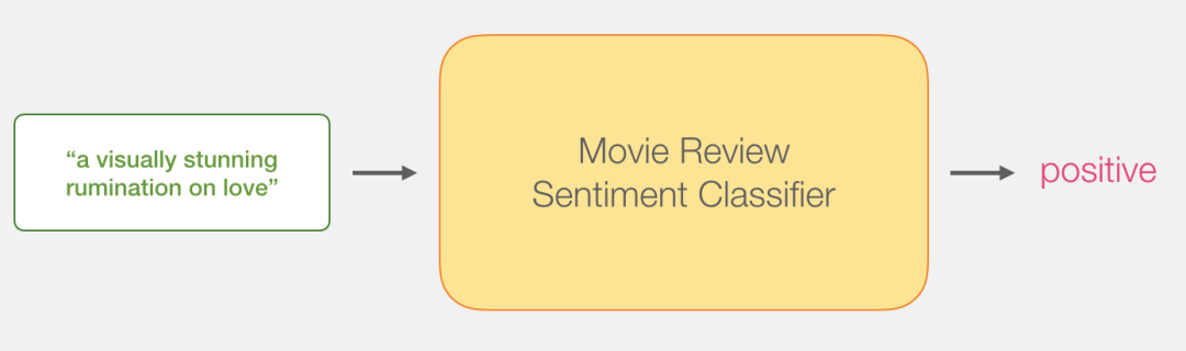
Model:Sentence Sentiment Classification
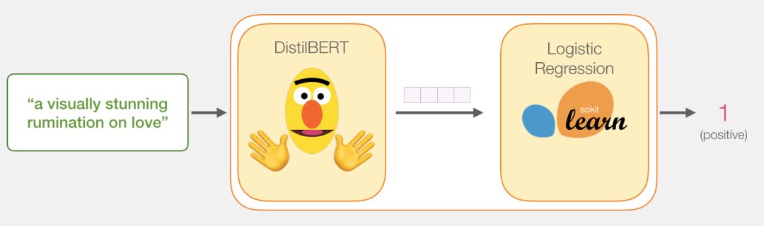
Our goal is to create a classifier that takes a sentence (similar to those in the dataset) as input and outputs a 1 (indicating that the sentence exhibits positive sentiment) or 0 (indicating that the sentence exhibits negative sentiment).The overall framework is shown in the figure below:
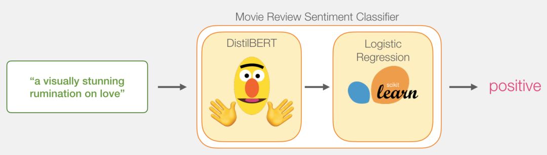
In fact, the entire model consists of two sub-models:
-
DistilBERT processes the sentence first and passes the extracted information to the next model.DistilBERT is a smaller version of BERT, developed and open-sourced by a team at HuggingFace.It is a more lightweight and faster model while achieving nearly the same performance as the original BERT.
-
The other model is a logistic regression model from scikit-learn, which receives the results processed by DistilBERT and classifies the sentences as positive or negative (0 or 1).
The data passed between the two models is a 768-dimensional vector.We can think of this vector as a sentence embedding that can be used for classification tasks.
If you have read my previous article about Illustrated BERT (https://jalammar.github.io/illustrated-bert/), this vector is actually the result at the first position with the input of the token [CLS].
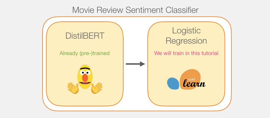
Although the entire model contains two sub-models, we only need to train the logistic regression model.As for DistillBERT, we will directly use the pre-trained model on English.However, this model does not need to be trained or fine-tuned to perform sentence classification.The general objective during BERT’s training has already given us some sentence classification capability, especially the output for the first position (which corresponds to [CLS]).I believe this is mainly due to BERT’s second training objective—Next Sentence Prediction.This objective seems to encapsulate sentence-level information in the output for the first position.The Transformers library provides us with an implementation of DistilBERT and pre-trained models.
The plan for this tutorial is as follows:We will first use the pre-trained DistilBERT to generate embeddings for 2,000 sentences.
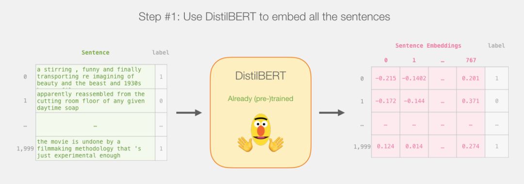
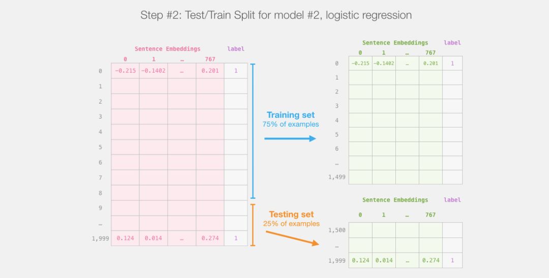
After that, we will no longer involve DistilBERT.The rest will be the work of Scikit Learn, and what we need to do next is to split the dataset into training and testing sets.
After dividing the output of DistilBERT (model #1) into training and testing sets, we have our dataset for training and evaluating logistic regression (model #2).Please note that in practice, sklearn shuffles the samples before splitting them into training and testing sets, rather than simply taking the first 75% in the original order.
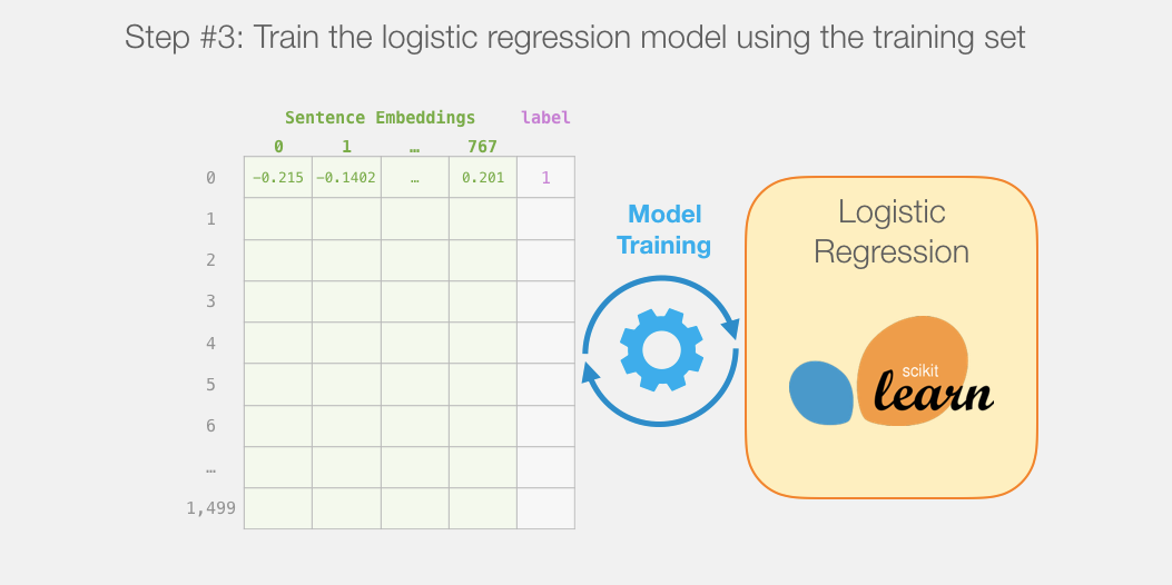
Next, we will train the logistic regression model on the training set:
How are the predicted values calculated?
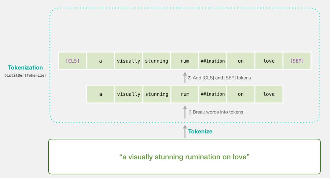
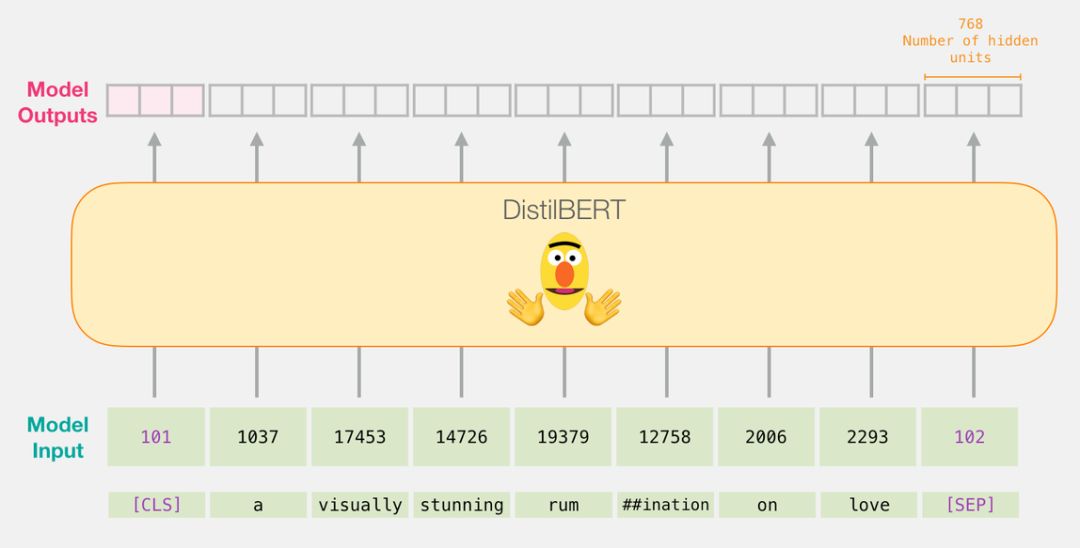
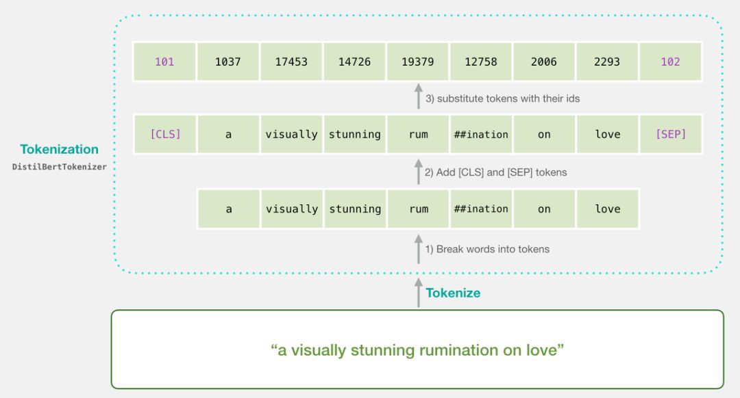
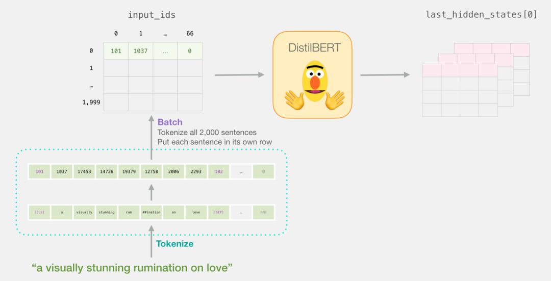
Before we delve into the code for training the model, let’s first look at how the trained model calculates its predicted values.Suppose we are classifying the sentence “a visually stunning rumination on love”.The first step is to use the BERT tokenizer to tokenize these words.Then, we add the special tokens required for sentence classification (adding [CLS] at the beginning and [SEP] at the end of the sentence).
The third step for the tokenizer is to look up and replace these tokens with their corresponding IDs in the embedding table, which we can obtain from the pre-trained model.If you are not familiar with word embeddings, please refer to “The Illustrated Word2vec”:
https://jalammar.github.io/illustrated-word2vec/.
Note that all the work of the tokenizer can be done with just one line of code:
tokenizer.encode("a visually stunning rumination on love", add_special_tokens=True)
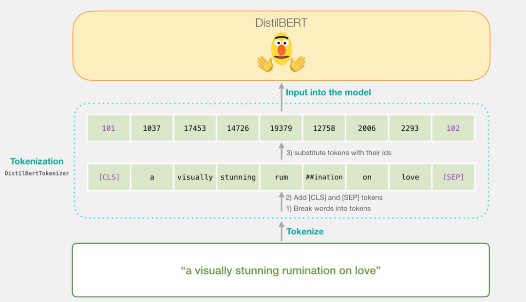
Now, the input sentence is in a format that can be passed to DistilBERT.
If you have read “Illustrated BERT” (https://jalammar.github.io/illustrated-bert/), this step can also be visualized as shown below:
Once the input vector is passed to DistilBert, the way it works is the same as in BERT, where each input word receives an output vector consisting of 768 floating-point numbers.
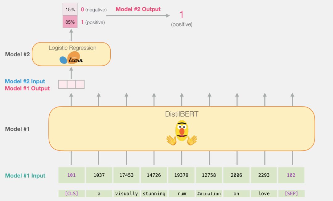
Since this is a sentence classification task, we only care about the first vector (the one corresponding to [CLS]).
This vector is what we will input to the logistic regression model.
From this point on, the task of the logistic regression model is:To classify this vector based on the experience it learned during the training phase.We can think of the entire prediction process like this:
We will discuss the entire training process and its related code in the next section.
In this section, we focus on the code for training this sentence classification model.Readers can obtain all the notebook code needed to complete this task from Colab and GitHub (links provided in the second paragraph of this article).
First, we need to import the relevant packages.
import numpy as np
import pandas as pd
import torch
import transformers as ppb # pytorch transformers
from sklearn.linear_model import LogisticRegression
from sklearn.model_selection import cross_val_score
from sklearn.model_selection import train_test_split
The link to the dataset is as follows:https://github.com/clairett/pytorch-sentiment-classification/.We can directly import it as a pandas DataFrame.
df = pd.read_csv('https://github.com/clairett/pytorch-sentiment-classification/raw/master/data/SST2/train.tsv', delimiter='\t', header=None)
We can check the content of the first five rows of the DataFrame using “df.head()”:
df.head()
The output is as follows:
Import Pre-trained DistilBERT Model and Tokenizer
model_class, tokenizer_class, pretrained_weights = (ppb.DistilBertModel, ppb.DistilBertTokenizer, 'distilbert-base-uncased')

## Want BERT instead of distilBERT? Uncomment the following line:
#model_class, tokenizer_class, pretrained_weights = (ppb.BertModel, ppb.BertTokenizer, 'bert-base-uncased')#

Load pretrained model/tokenizer
tokenizer = tokenizer_class.from_pretrained(pretrained_weights)
model = model_class.from_pretrained(pretrained_weights)
Now, we can perform tokenization on the dataset.Please note that what we are doing here is slightly different from the examples above.The previous example only tokenized and processed one sentence.Here, we will tokenize and process all sentences as the same batch.In the notebook, considering computational power, we only used 2,000 sentences.
tokenized = df[0].apply((*lambda* x: tokenizer.encode(x, add_special_tokens=True)))
The code above converts all sentences into a list of IDs.
Now, the dataset has become a list of lists (or Pandas arrays and DataFrames).Before DistilBERT can process them as input data, we need to arrange these vectors into the same dimension (padding shorter sentences with the ID “0”).You can see the code for the “padding” operation in the notebook, which involves simple operations with Python strings and arrays.
After completing the “padding” operation, we will have a matrix/tensor that BERT can accept.
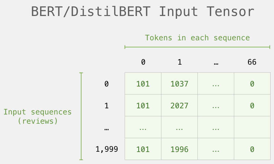
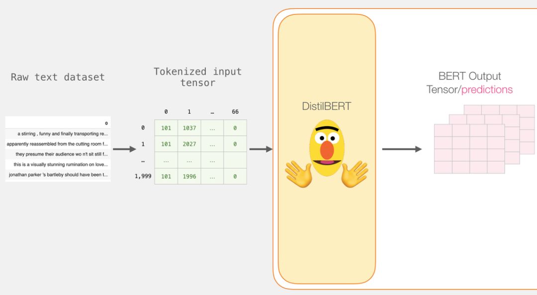
Now, we create an input tensor based on the padded token matrix and pass it to DistilBERT
input_ids = torch.tensor(np.array(padded))

with torch.no_grad():

last_hidden_states = model(input_ids)
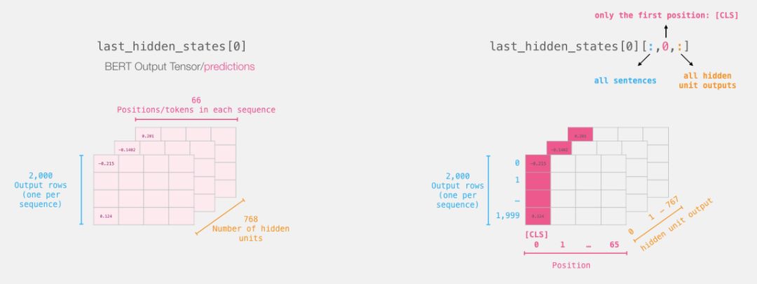
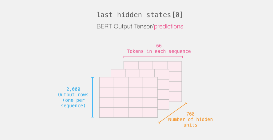
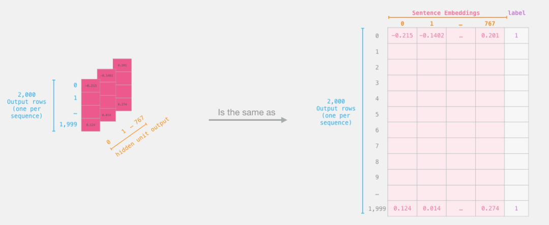
After this step, the output of DistilBERT will be assigned to “last_hidden_states”. This is a tuple with dimensions (number of sentences, maximum number of words in the sequence, number of hidden layers in the DistilBERT model).In this example, the dimension is (2000, 66, 768) because we have 2000 sentences, and the longest sequence length among these sentences is 66, with 768 hidden layers in the DistilBERT model.
Expanding the Output Tensor of BERT
Next, we need to expand this three-dimensional output tensor.We can first analyze its dimensions:
Reviewing the ‘Life’ of These Sentences
Each row represents a sentence in the dataset.The processing of the first sentence is shown in the figure below:
Slicing to Get Important Parts
For the sentence classification task, we are only interested in the output corresponding to [CLS] from BERT, so we only keep the slice corresponding to [CLS] from the “cube” and discard the other content.
This is how we obtain the two-dimensional tensor we need from the three-dimensional tensor:
 # Slice the output for the first position for all the sequences, take all hidden unit outputs
 features = last_hidden_states[0][:,0,:].numpy()
Now, “features” is a two-dimensional numpy array that contains the embeddings of all sentences in our dataset.
The tensor obtained by slicing the output from BERT.
Dataset for Logistic Regression
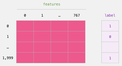
Now that we have obtained the output from BERT and assembled the dataset for training the logistic regression model.These 768 columns are features, and we also provided the labels from the original dataset.
We have a labeled dataset for training logistic regression.These features correspond to the part of BERT that corresponds to [CLS] (position #0), which is the part we obtained by slicing in the previous image.Each row corresponds to one sentence in the dataset, and each column corresponds to the hidden units in the feedforward neural network of the top transformer module in the BERT/DistilBERT model.
After completing the traditional training/test split operation in machine learning, we can create our own logistic regression model and train it with our dataset.
labels = df[1]
train_features, test_features, train_labels, test_labels = train_test_split(features, labels)
The code above splits the dataset into training and testing sets:
Next, we will train the logistic regression model on the training set.
lr_clf = LogisticRegression()
lr_clf.fit(train_features, train_labels)
Now the model has been trained, and we can evaluate it using the test set.
lr_clf.score(test_features, test_labels)
The output of the above code tells us that this model achieved an accuracy of 81%.
As a reference, the highest accuracy that can be achieved on this dataset is 96.8.In this task, we can also train DistilBERT to improve its score, which is commonly referred to as the fine-tuning process, which can update BERT’s weight parameters and allow it to achieve better performance in sentence classification tasks (commonly referred to as “downstream tasks”).After fine-tuning, DistilBERT can achieve an accuracy of 90.7, while the full BERT can achieve 94.9.
The relevant notebook code link was provided at the beginning of this article, go explore it yourself!
This concludes the content of this article, which should be very suitable for those encountering BERT for the first time.The next step is to check the documentation and try to fine-tune it.You can also go back and convert DistilBERT in the code to BERT and see how it works.
Machine Heart “SOTA Models”:22Big fields, 127 tasks, machine learning SOTA research all in one.
ClickRead the original textto visit immediately.