Basic Principles of Neural Networks and Implementation in Python

1. Basic Principles of Neural Networks

1. Simple Principles of Biological Neural Networks

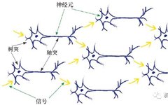
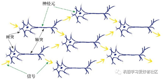
In biological neural networks, each neuron’s dendrite receives electrical signals from multiple previous neurons, combining them into a stronger signal. If the combined signal is strong enough and exceeds the threshold, the neuron will be activated and will also send out a signal, which will travel along the axon to the terminal of this neuron, passing on to the dendrites of subsequent neurons, as shown in Figure 1.

2. Basic Principles of Artificial Neural Networks

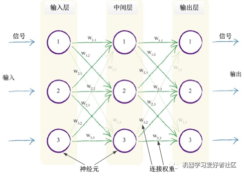
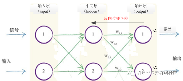
Inspired by biological neural networks, multi-layer artificial neural networks are constructed, where each layer’s artificial neurons are interconnected with neurons from the previous and next layers, as shown in Figure 2. Each connection displays the relevant connection weights, where smaller weights weaken the signal, while larger weights amplify the signal.

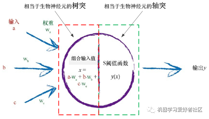
For a single neuron in the neural network, the front half of the artificial neuron (the red dashed box in Figure 3) corresponds to the dendrite of a biological neuron, serving as the input end to receive signals from multiple neurons and combine them; the back half of the artificial neuron (the green dashed box in Figure 3) corresponds to the axon of a biological neuron, serving as the output end to send signals to more neurons; the boundary between the front and back ends is the activation function, which corresponds to the threshold function of a biological neuron, used to determine if the combined input signal reaches the threshold. If it does, the neuron activates and outputs a signal; otherwise, it suppresses the signal and does not output.

Thus, the basic principle of neural networks is to compare the output value y of the neural network with the true output value labeled in the training samples, calculate the output error, and then use this error to guide the adjustment of connection weights between each pair of neurons in the two layers, gradually improving the output value of the neural network until the error between it and the true output value of the training samples is minimized and falls within an acceptable range. It can be seen that the connection weights between each pair of neurons in the two layers are the content that the neural network needs to learn. Continuous optimization of these connection weights is necessary to improve the network’s output and achieve satisfactory results.

3. Forward Calculation of Neural Network Output

As shown in Figure 2, once input signals enter the neural network from the first layer (the input layer), regardless of how many layers are beyond the input layer, the output signals through each layer can be calculated using the following two steps: first, adjust the signals input from each neuron in the previous layer using the connection weights and combine them; second, apply the activation function to the combined signal to generate the output signal for that layer. For the input layer, it only represents the input for each neuron in the input layer, and no activation function is used for the neurons in the input layer. Therefore, to represent the forward output values of each layer of the neural network after the input layer using powerful matrix operations, it can be expressed as:

Where formula (1) adjusts and combines the signals input from each neuron in the previous layer, resulting in a combined signal vector, where W is the connection weight matrix between the neurons of this layer and the previous layer, and X is the input signal vector from the previous layer; formula (2) applies the activation function to the combined signal and generates the output signal for that layer, which is the output signal vector of that layer, and f is the chosen activation function (the threshold function).

4. Backpropagation of Errors in Neural Networks

As shown in Figure 2, when we propagate signals from the input layer to the output layer in the neural network, we use the connection weights. In addition, when the errors obtained from the output layer are backpropagated to each intermediate layer, we also need to use the connection weights. Similar to the forward propagation of input signals, we assign larger errors to connections with larger connection weights. Therefore, during the error backpropagation process, the calculation of errors for nodes in the intermediate layer (also known as the hidden layer) is that the error for each node in the intermediate layer is the sum of the errors divided by all the connection weights in the forward connections of that node.

For example, in the neural network shown in Figure 4, the error of the first neuron (also called a node) in the intermediate layer receives a portion of the output error from the first output node through the weight connection, and also a portion from the second output node’s output error; its error is the sum of these two parts of errors. Similarly, the error of the second node in the intermediate layer is also obtained by summing the errors divided by connection weights. Therefore, the errors of the intermediate layer nodes calculated through the backpropagation of errors can be expressed in matrix form as:

Observing the above equation, the errors of the intermediate layer nodes can be seen as obtained from the weight matrix and the output layer errors through matrix multiplication. Here, each element of the weight matrix in this formula is a fraction, where the denominator is a normalization factor. If we ignore these normalization factors for each fraction, only the size of the calculated intermediate layer node errors is affected, while it still complies with the principle that larger connection weights mean carrying larger output errors to the intermediate layer. At this point, the equation simplifies to:

In this case, the weight matrix in this equation is the connection weight matrix in formula (1) of the forward calculation output of the neural network. Therefore, to continue using powerful matrix operations to represent the intermediate layer error values obtained during the backpropagation of errors from the output layer, it can be expressed as:

Where formula (3) is the error vector of the intermediate layer nodes, W is the connection weight matrix between the output layer and the intermediate layer (if there are multiple layers in between, it is the connection weight matrix between the last layer and that intermediate layer), and E is the error vector of the output layer (if there are multiple layers in between, it is the error vector of the last layer).

5. Updating Connection Weights in Neural Networks

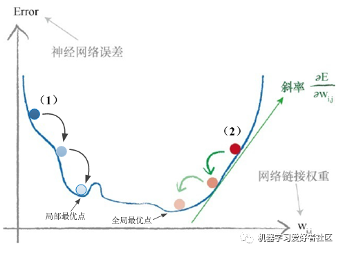
How to update the connection weights between the input layer and the intermediate layer, as well as between the intermediate layer and the output layer, is a core issue in the learning process of neural networks. From formula (3), we know that the error of the neural network is a function of the connection weights. Thus, improving the neural network means reducing this error by changing the connection weights. Therefore, in the process of minimizing the error, we need to use the gradient descent method to calculate the slope of the error function concerning the connection weights.

As shown in Figure 5, during the gradient descent process, (1) and (2) represent two different starting points. In case (1), it is easy to get trapped in a local optimum without finding the connection weights that minimize the error. Therefore, to avoid this issue, different starting connection weights will be used in the neural network for gradient descent to seek the global optimum.

Therefore, obtaining the slope of the error function concerning the connection weights is particularly crucial, as this slope indicates the direction in which the gradient descent method will minimize the output error value. For the i-th node, the direction of change for the connection weight from the j-th node in the previous layer is opposite to the slope direction; its updating formula is:

Next, we will focus on calculating the slope. For the i-th node, its output value is y, and the true output value is t (which is a real constant), so the slope formula is:

And the derivative formula of the S function is: . Therefore, formula (5) can be written as:

Observing the above equation, we find that the obtained slope formula consists of three parts multiplied together: the first part is the error value, but we omitted the factor of 2 when deriving this formula because we are only interested in the slope of the error function, so we need not concern ourselves with its numerical value; the second part is the output value of the node obtained from the forward calculation of the neural network using formulas (1) and (2); the third part is the output of the j-th node in the previous layer connected to the i-th node.

Therefore, whether it is the slope of the error function concerning the connection weights between the input layer and the intermediate layer or between the intermediate layer and the output layer, both can be calculated using formula (6). However, in the process of calculating the slope of the error function concerning the connection weights between the input layer and the intermediate layer, we need to first use the neural network backpropagation error represented by formula (3) to obtain the errors of the intermediate layer before we can get the error value represented in the first part of formula (6). In contrast, in the process of calculating the slope of the error function concerning the connection weights between the intermediate layer and the output layer, we can directly obtain the error value represented in the first part of formula (6) from (true value – output value). Therefore, to continue representing the updating connection weight matrix described by the slope matrix of the error function using powerful matrix operations, it can be expressed as:

2. Python Neural Network Programming

1. Code Framework for a Three-Layer Neural Network

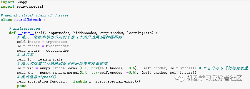
Based on the basic principles of neural networks and the relevant calculation formulas described above, a three-layer neural network can be created using Python, without limiting the number of nodes in each layer. Therefore, a neural network class should include at least the following three functions:

1. Initialization function – set the number of nodes in the input layer, intermediate layer, and output layer, set the learning rate, and randomly initialize the connection weight matrices between the input layer and the intermediate layer and between the intermediate layer and the output layer.

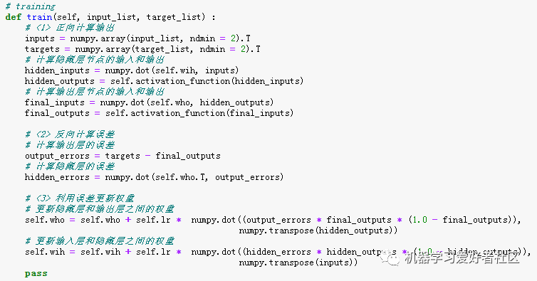
2. Training function – after providing the training set samples, forward calculate the output value and compute the error value based on the true values labeled in the samples, then backpropagate the error to calculate the error values of the intermediate layer, and finally calculate the slope of the error function concerning the connection weights and update the connection weight matrices between the input layer and the intermediate layer and between the intermediate layer and the output layer using gradient descent.

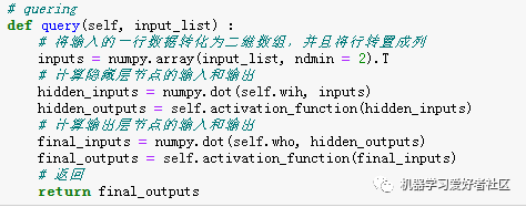
3. Query function – after providing input, calculate the forward output values of each layer of the neural network and output the final value of the neural network.

Based on the above code framework, the specific code for the neural network class is provided below:

2. Training Neural Networks Using the MNIST Handwritten Digit Dataset

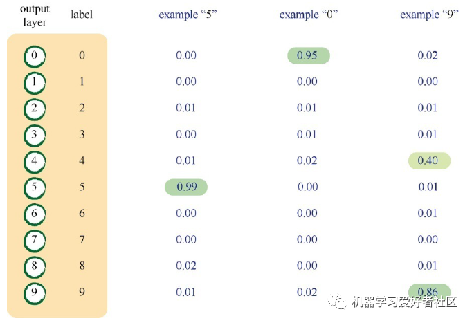
Since each handwritten digit in the MNIST dataset has pixels uniformly represented by grayscale values, the number of input layer nodes needs to correspond to this, set to 784. For the output layer, it needs to recognize and output one of the ten digits from 0 to 9, which means the neural network should have 10 output layer nodes, each corresponding to a digit label.

For instance, in Figure 9, if the neural network recognizes the handwritten digit as “5”, the 6th node in the output layer is activated, while the other output nodes remain suppressed; if the neural network recognizes the handwritten digit as “0”, the 1st node in the output layer is activated, while the other output nodes remain suppressed; if the neural network recognizes the handwritten digit as “9”, the 10th node in the output layer is activated, while the other output nodes remain suppressed.

Of course, suppressed nodes do not necessarily output particularly small signals; they simply have relatively smaller signal values compared to activated nodes, as we typically only consider the node with the largest signal value as the activated node.

Additionally, we use the same training dataset and repeat the training multiple times to enhance the performance of the neural network. We refer to one training cycle as one generation; thus, training for 5 generations means running the program with the entire training dataset 5 times. Although this approach increases the computer’s running time, it is worthwhile. This is because, as mentioned in the basic principles of neural networks, the connection weight matrix is randomly initialized, which means that different starting points in the gradient descent process provide more opportunities to descend and are less likely to get trapped in incorrect local optima, making it more conducive to updating connection weights in the gradient descent process. Therefore, the code for training the neural network using the MNIST handwritten digit dataset is as follows:

3. Testing the Neural Network with Handwritten Digits

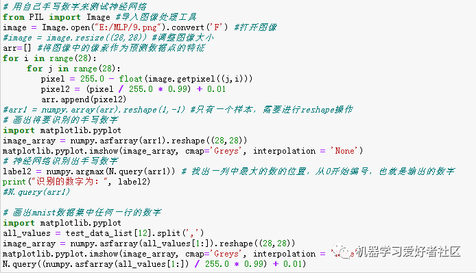
Once the neural network has completed training, we can also use the MNIST test dataset to evaluate the neural network’s performance, checking the recognition accuracy of the trained neural network on the test dataset composed of handwritten digits it has never seen before. Additionally, we can write a few digits by hand, create images, and import them into the neural network program to observe whether the trained neural network can correctly recognize them. Thus, the code for testing the trained neural network using the MNIST test dataset is shown in Figure 11, and the code for testing the trained neural network with our handwritten digits is shown in Figure 12:

The output of the test results is shown in the following figure:

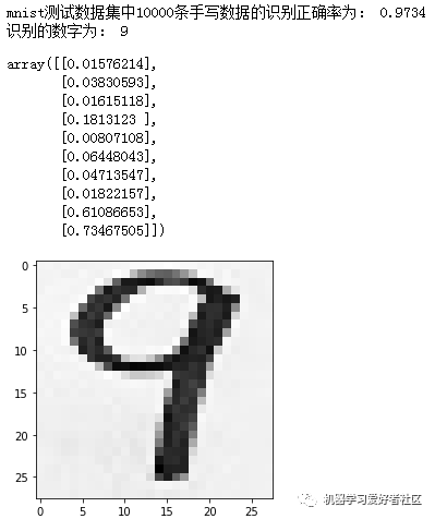
As can be seen from the above figure, the constructed neural network performs exceptionally well on the MNIST test dataset, achieving approximately 97% accuracy in recognizing handwritten digits in the MNIST test dataset. Furthermore, the neural network was also able to correctly identify the handwritten digit “9” we wrote ourselves, as indicated by the highest signal value among the 10 output nodes in the output layer, confirming that this node is the activated one, thus the digit label “9” is the final recognition result given by the neural network.

In conclusion, this article has introduced the basic principles of neural networks, core calculation formulas, and corresponding Python code, and has also successfully recognized our handwritten digits using the trained neural network model, marking a good starting point for learning about neural networks.