Source: Deephub Imba


This article is about 4500 words long and is recommended for a 5-minute read.
This article describes a method for training high-quality, transferable embeddings using self-supervised learning techniques on user search data from within the website.
The number of categories in large websites is vast, and manual tagging is generally unfeasible. Therefore, understanding the content of large catalogs poses a significant challenge for online businesses, making it very difficult for new product discovery. However, this problem can be addressed using self-supervised neural network models.
In the past, we relied on manual tagging of products within the system. While this did solve the problem, it incurred a significant labor cost. If we could create a universal machine learning-based method to semantically auto-associate products and gain a deeper understanding of the existing catalog content, we could automate product recommendations, search, promotional activities, and operational intelligence.
This article describes a method for training high-quality, transferable embeddings using self-supervised learning techniques on user search data from within the website. Additionally, this article lists some alternative methods and details the model training and evaluation process of our chosen solution, comparing the advantages and disadvantages of each approach.
Category Issues for Large Websites
For large websites, the content of the site’s catalog is not static. When we add new categories, a new model needs to be trained for machine learning. Is there a way to handle the catalog without building a custom model? First, understanding the content of categories is crucial for operational business and consumer-facing content searches because:
-
Categories can be recommended based on known consumer preferences.
-
Products can be recommended to consumers when they interact with new stores.
-
More relevant stores and products can be recommended during search queries.
-
Similar promotions to consumers’ recent order history can be automatically recommended.
-
Understanding what items consumers purchase after searching.
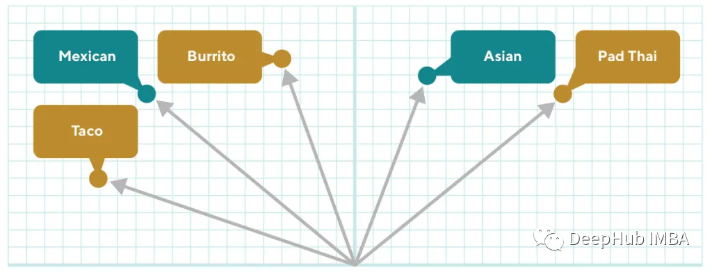
An example of queries (green) and product (yellow) representations in the same latent space. We want to learn an embedding representation where lines of the same color have high cosine similarity (small angles between them), while lines of different colors have low cosine similarity (large angles between them). This means we need to encode queries and items into the same space and learn high-quality representations for both.
In the context of search, we also want to create a queryable embedding that can be compared with product and store embeddings. The model needs to place queries and products in the same latent space (as shown in Figure 1) for comparability. Once the query “mexican” and the product “taco” are embedded, the embedding space can tell us that they are related (cosine similarity). We also need to embed stores and buyers in the same latent space, allowing us to use embedding methods that include catalog knowledge for store recommendations.
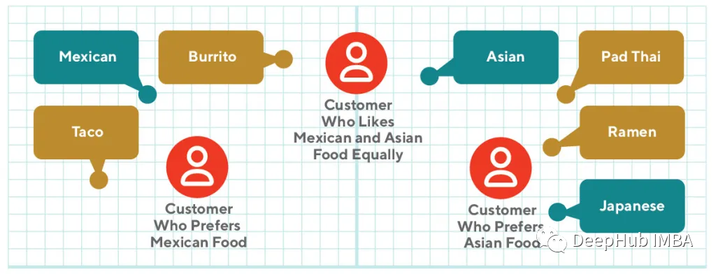
By defining consumer embeddings (blue) as the average of their product embeddings (green), we can understand different preferences of consumers. In the above figure, consumers who frequently purchase Mexican cuisine are closer to Mexican dishes than those who frequently purchase Asian cuisine. Consumers who buy both types of food will form an embedding between the clusters of Mexican and Asian foods.
Therefore, the problem we want to solve is how to effectively train on very rare categories using limited labeled data, which requires leveraging self-supervised methods to train embeddings. But before we begin, let’s review traditional techniques for training embeddings to understand why they cannot solve the problem.
Review of Techniques for Building Embeddings
For the above use case, traditional methods include training Word2vec on entry IDs or training deep learning classifiers and taking the output of the last linear layer. In natural language processing (NLP), fine-tuning large pre-trained models like BERT has also become common. However, for the ever-evolving and sparse catalog problem, we will introduce these methods one by one:
Solution 1: Embedding Word2vec on Entity IDs
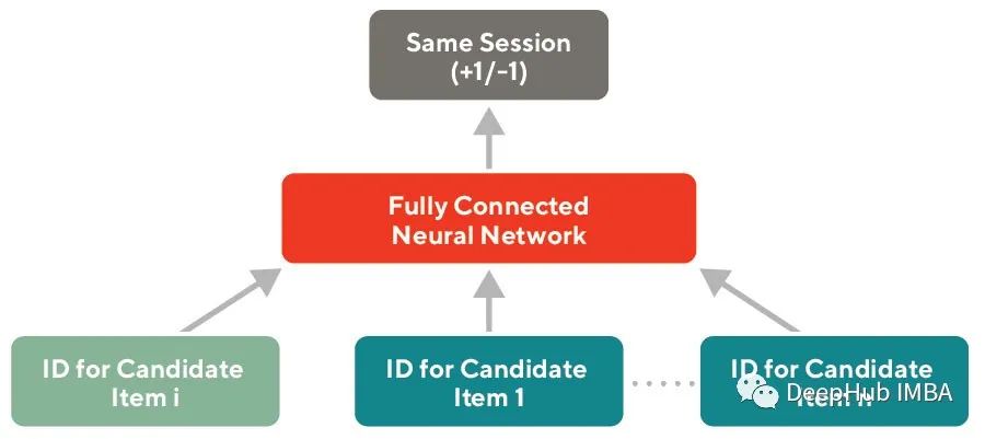
Word2vec embeddings can be trained on any set of entity IDs based on customer behavior such as visits or purchases. These embeddings learn relationships between IDs by assuming that entities interacting with customers in the same session are related to each other, similar to the distribution assumption of Word2vec. Store and customer behaviors regularly train this type of embedding for use in recommendations and other personalization applications. See the figure below:
Word2vec embeddings have some drawbacks in retaining semantic similarity for large catalogs. When new entities are added to the catalog, they need to be retrained regularly. If millions of products are added daily, retraining these embeddings every day is computationally expensive. Embeddings trained using this method are also prone to sparsity issues, as IDs that interact with customers infrequently are not well-trained.
Solution 2: Training Embeddings with Supervised Task-Based Deep Neural Networks
Deep neural networks trained on classification tasks have lower training errors and can learn high-quality target class representations. The output of the last hidden layer of the network can be viewed as the embedding of the original input. For diverse and large high-quality labeled datasets, this method can effectively learn high-quality embeddings and can be reused in classification tasks.
 This training method does not always guarantee that the underlying embeddings have good metric properties. Since our priority is the usability of downstream applications, we hope that these embeddings can be easily compared using simple metrics like cosine similarity. Because this method requires supervision, the quality of the learned metrics largely depends on the quality of the training set’s annotations. We need to ensure that the dataset has good negative samples to ensure the model can learn to distinguish closely related labels. This issue becomes particularly severe for rare classes with limited data samples. Thus, unsupervised solutions can circumvent this problem by automatically generating samples from unlabeled data and learning representations of the labels.
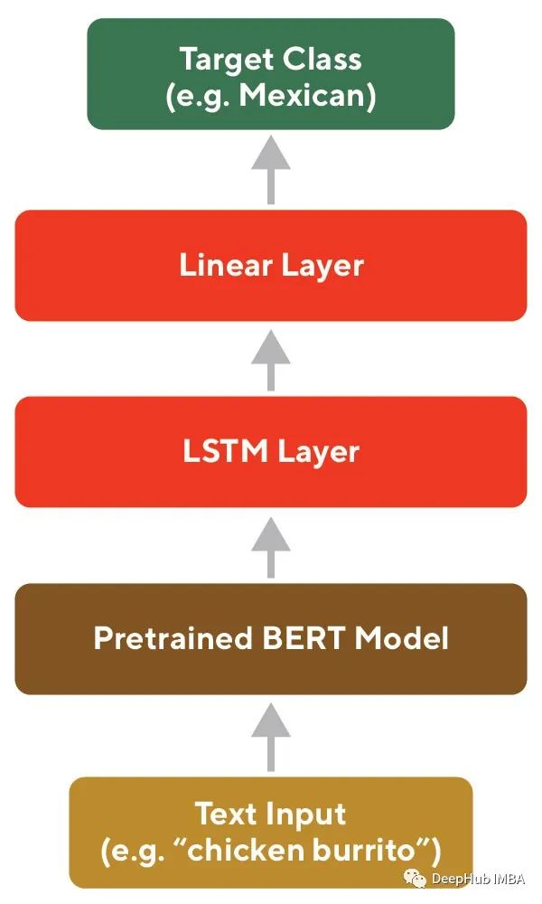
Solution 3: Fine-tuning a Pre-trained Language Model like BERT
With recent advances in training large NLP models on large corpora, fine-tuning these models through transfer learning for task-specific embeddings has become a popular method (as exemplified in the architecture shown in Figure 5). BERT is a popular pre-trained model, and this method can be implemented directly using open-source libraries, overcoming the data sparsity issue and serving as a very good baseline model.
While BERT embeddings represent a significant improvement over the baseline, their training and inference are very time-consuming due to the model’s size. Even using distilled models (like DistilBERT or ELECTRA), they may be much slower than much smaller custom models. Additionally, if there is a sufficient amount of domain-specific data, even if it is unlabeled, self-supervised methods can have better metric properties for specific tasks compared to pre-trained language models.
This training method does not always guarantee that the underlying embeddings have good metric properties. Since our priority is the usability of downstream applications, we hope that these embeddings can be easily compared using simple metrics like cosine similarity. Because this method requires supervision, the quality of the learned metrics largely depends on the quality of the training set’s annotations. We need to ensure that the dataset has good negative samples to ensure the model can learn to distinguish closely related labels. This issue becomes particularly severe for rare classes with limited data samples. Thus, unsupervised solutions can circumvent this problem by automatically generating samples from unlabeled data and learning representations of the labels.
Solution 3: Fine-tuning a Pre-trained Language Model like BERT
With recent advances in training large NLP models on large corpora, fine-tuning these models through transfer learning for task-specific embeddings has become a popular method (as exemplified in the architecture shown in Figure 5). BERT is a popular pre-trained model, and this method can be implemented directly using open-source libraries, overcoming the data sparsity issue and serving as a very good baseline model.
While BERT embeddings represent a significant improvement over the baseline, their training and inference are very time-consuming due to the model’s size. Even using distilled models (like DistilBERT or ELECTRA), they may be much slower than much smaller custom models. Additionally, if there is a sufficient amount of domain-specific data, even if it is unlabeled, self-supervised methods can have better metric properties for specific tasks compared to pre-trained language models.
Training Embeddings via Self-Supervised Learning
After researching the above methods, we used a self-supervised approach to train embeddings based on category names and search queries. By using subword information, such as character-level information, these embeddings can also generalize to texts that do not appear in the training data.
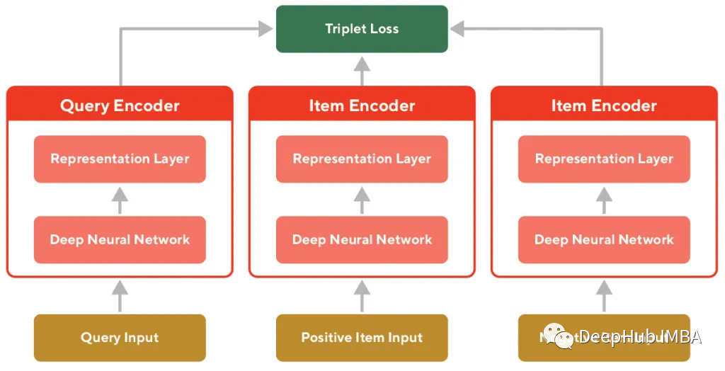
To ensure good metric performance, we employed a Siamese Neural Network architecture with triplet loss. The triplet loss attempts to push similar samples together in the latent space while separating different samples. The Siamese Neural Network ensures that the encodings used for query and product texts are embedded into the same latent space in a way that maintains distance between similar examples.
To train the triplet loss, we need a dataset structured as . The anchor is defined as the original query text, and the “relevant” and “irrelevant” items for the query are treated as positive and negative, respectively.
To construct this dataset (as shown in the example in Figure 6), a set of heuristic methods needs to be developed to formulate training tasks. The following heuristic methods are used to determine the relevant and irrelevant items corresponding to positive and negative training samples:
If a user searches for query Q and then immediately purchases item X in the same session, where X is the most expensive item in the shopping cart, then item X is relevant to query Q.
This heuristic method for positive samples ensures that we only take the main items from the shopping cart that we consider to be the most relevant.
If X was purchased in query R and the Levenshtein distance between Q and R is > 5, then item X is irrelevant to query Q.
This heuristic method for negative samples ensures that items purchased for similar queries (e.g., “burger” and “burgers”) are not considered irrelevant. Generating high-quality negative samples is crucial to preventing mode collapse. In this example, even such simple heuristics and natural variations in text are sufficient for training, but there may be better methods that require further exploration.
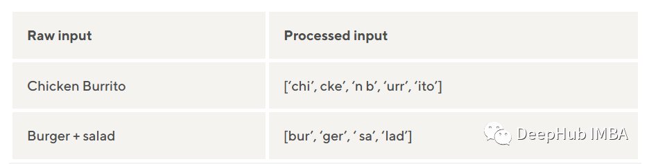
We also performed minimal normalization on the input, converting all strings to lowercase and removing punctuation. This allows the trained model to adapt to spelling errors and other natural variations in language.
To ensure the model can generalize to out-of-vocabulary labeled samples, we used character trigrams to handle the input.
We experimented with various alternative tokenization schemes (word n-grams, byte pair encoding, WordPiece, and word + character n-grams) but found that trigrams had similar or better predictive performance and could be trained faster.
The model is a Siamese network (as shown in Figure 8), which uses encoders consisting of deep neural networks and outputs the final embeddings through a linear layer. All weights are shared between the encoders. Since weights are shared between encoders, all heads’ encodings enter the same latent space. The output of the encoder is used to compute the triplet loss.
The loss is computed as follows:
L(a, p, n, margin) = max(d(a, p) -d(a, n) + margin, 0)
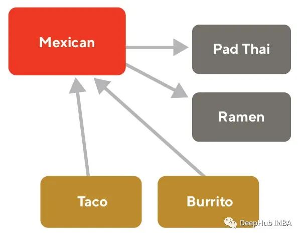
For the query “Mexican” (red), the triplet loss attempts to bring the positive embedding (yellow) closer and separate the negative (gray).
Sample code for the neural network. Here we extract details of the encoder to illustrate how to compute forward propagation and loss.
class SiameseNetwork(torch.nn.Module):  def __init__(self, learning_rate, transforms, model, **kwargs):      super().__init__()
      self.learning_rate = learning_rate      self.transforms = transforms      self._encoder = model(**kwargs)      self.loss = torch.nn.TripletMarginLoss(margin=1.0, p=2)
  def configure_optimizers(self):      return torch.optim.Adam(self.parameters(), lr=self.learning_rate)
  def _loss(self, anchor, pos, neg):      return self.loss(anchor, pos, neg)
  def forward(self, anchor, seq1, seq2):      anchor = self._encoder(anchor)      emb1 = self._encoder(seq1)      emb2 = self._encoder(seq2)      return anchor, emb1, emb2
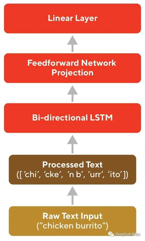
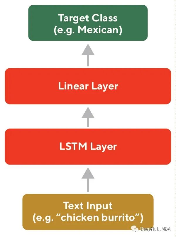
The actual encoder architecture is a bidirectional LSTM followed by a linear layer. The LSTM is responsible for processing a series of characters into vectors.
Below is the code for the encoder:
class LSTMEncoder(torch.nn.Module):  def __init__(self, output_dim, n_layers=1, vocab_size=None, embedding_dim=None, embeddings=None, bidirectional=False, freeze=True, dropout=0.1):      super().__init__()      if embeddings is None:          self.embedding = torch.nn.Embedding(vocab_size, embedding_dim)      else:          _, embedding_dim = embeddings.shape          self.embedding = torch.nn.Embedding.from_pretrained(embeddings=embeddings, padding_idx=0, freeze=freeze)
      self.lstm = torch.nn.LSTM(embedding_dim, output_dim, num_layers=n_layers, bidirectional=bidirectional, dropout=dropout, batch_first=True)      self.directions = 2 if bidirectional else 1
      self._projection = torch.nn.Sequential(          torch.nn.Dropout(dropout),          torch.nn.Linear(output_dim * self.directions, output_dim),          torch.nn.BatchNorm1d(output_dim),          torch.nn.ReLU(),          torch.nn.Linear(output_dim, output_dim),          torch.nn.BatchNorm1d(output_dim),          torch.nn.ReLU(),          torch.nn.Linear(output_dim, output_dim, bias=False),      )
  def forward(self, x):      embedded = self.embedding(x) # [batch size, sent len, emb dim]      output, (hidden, cell) = self.lstm(embedded)      hidden = einops.rearrange(hidden, '(layer dir) b c -> layer b (dir c)', dir=self.directions)      return self._projection(hidden[-1])
Model Evaluation
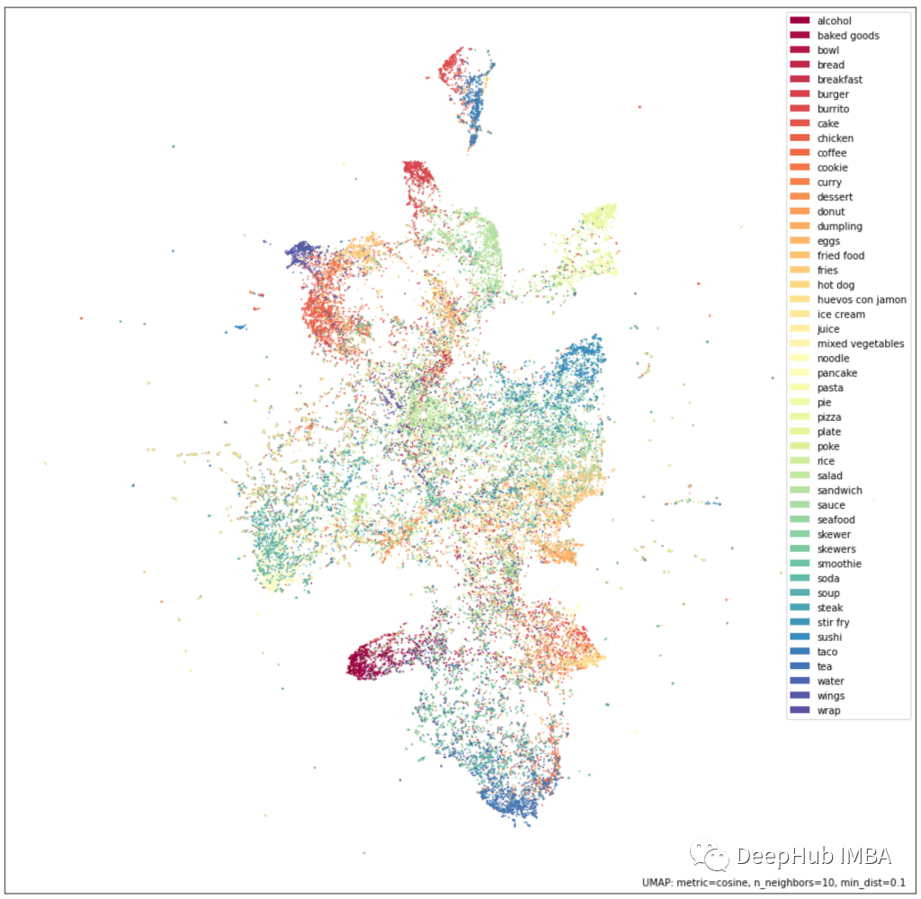
The model is evaluated based on qualitative metrics (such as evaluating the embedding UMAP projections) and quantitative metrics (such as baseline F1 scores). Qualitative results are assessed by observing the UMAP projections of the embeddings (as shown in the figure below). Similar classes can be seen projected near each other, indicating that the embeddings effectively capture semantic similarity.
Considering the good results from qualitative assessments, we also conducted more rigorous benchmarking on some baseline classification tasks to understand the quality of the embeddings and the potential benefits of using them in other internal models.
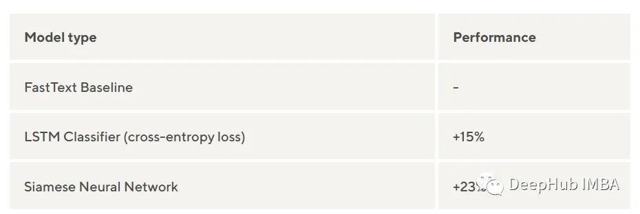
The model’s F1 score improved by about 23% over the baseline (FastText classifier). This is a significant improvement, especially since the Siamese neural network was evaluated on zero-shot classification tasks while the baseline was trained on labeled data.
Using these embeddings as features for downstream classification tasks can significantly improve sample efficiency. Training a model with the same accuracy using the FastText classifier requires more than three times the existing labeled data volume. This indicates that the learned representations carry a wealth of information about the text content.
Examples of Embedding Applications
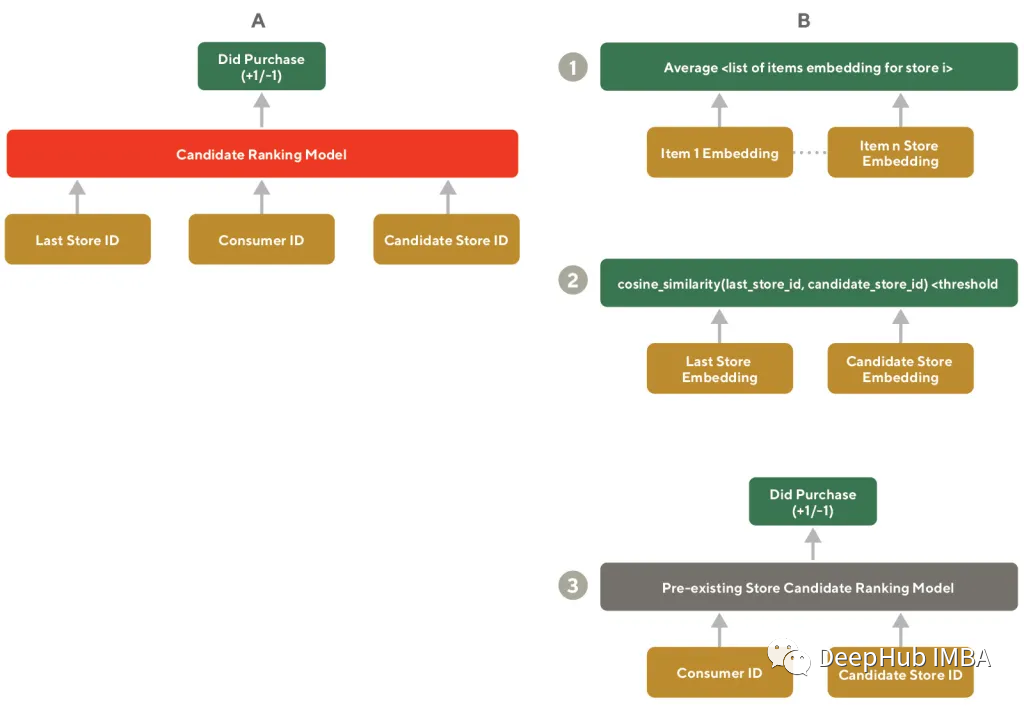
To improve content recommendations for customers, we recommend similar other stores based on the categories of stores that customers recently purchased from. Without embeddings, a dedicated model would need to be built that considers and attempts to predict the purchase rate for each candidate store_id. However, here we use the embeddings we have already generated, which requires two steps:
-
Retrieving stores similar to last_store_id from the already generated embeddings.
-
Using a ranker to personalize the ranking of filtered stores for each customer.
Since calculating cosine similarity is very fast, and we do not need to collect any other data for ranking, the figure below details this process. By averaging the product embeddings in each store, a semantic embedding for a store can also be easily generated, which can be done in batch processing, reducing the load on real-time systems.
Conclusion
Self-supervised methods are particularly useful for developing immediately reusable ML products in rapidly growing catalogs. While other ML methods may be more suited for specific tasks, self-supervised embeddings can still provide a strong baseline for tasks requiring high-quality text data representations. Compared to off-the-shelf embedding methods (like FastText or BERT), domain-specific embedding methods are often better suited for internal applications (such as search and recommendations).
References:
[1] Siamese Neural Networks for One-shot Image Recognition. https://www.cs.cmu.edu/~rsalakhu/papers/oneshot1.pdf
[2] A Simple Framework for Contrastive Learning of Visual Representations. https://www.cs.toronto.edu/~hinton/absps/simclr.pdf
[3] Deep Metric Learning with Triplet Loss. https://arxiv.org/pdf/1412.6622.pdf
[4] FaceNet: A Unified Embedding for Face Recognition and Clustering. https://arxiv.org/pdf/1503.03832.pdf
This article is an online practice sharing from DoorDash, and the original article can be found here:
https://doordash.engineering/2021/09/08/using-twin-neural-networks-to-train-catalog-item-embeddings/
Edited by: Wang Jing
Proofread by: Lin Yilin