An Overview of Graph Neural Networks (GNN): From Graphs to Graph Convolution

This article is about 8000 words long and is suggested to be read in 16 minutes.
This article provides a detailed introduction to the relevant content from Graph to Graph Convolution.

The author has recently reviewed several papers on Graphs and Graph Convolutional Neural Networks (GCNs) and is deeply impressed by their power. However, some surveys or tutorials assume that readers have a background knowledge of Graph Neural Networks, which may not be friendly to readers who have not studied signal processing. At the same time, many tutorials only explain what it is without discussing why it is so, nor do they clarify the differences and design motivations of different network structures.

Therefore, this article attempts to follow the historical context of Graph Neural Networks, starting from the earliest Graph Neural Networks (GNNs) based on fixed-point theory and gradually discussing the currently most popular Graph Convolutional Networks (GCNs), hoping to provide readers with some inspiration and insight.

1. The outline and key points of this article are mainly referenced from two surveys on Graph Neural Networks, namely A Comprehensive Survey on Graph Neural Networks by IEEE Fellow and Deep Learning on Graphs: A Survey from Professor Zhu Wenwu’s group at Tsinghua University. Here, I would like to express my respect to the authors of these two surveys.

2. At the same time, many of my understandings of some Graph Convolutional Networks in this article are inspired by highly upvoted answers to questions on Zhihu, and I am very grateful for their selfless sharing!3. Finally, this article also cites some vivid images from the Internet, and I would like to thank the authors of these images. The images not marked with sources in this article are all created by the author. If you need to reprint or quote, please contact me.

Historical Context

Before starting the main text, I would like to take everyone back to review the development history of Graph Neural Networks. However, because there are many branches in the development of Graph Neural Networks, some of my descriptions may not be comprehensive, and my opinions are for readers’ reference only:

1. The concept of Graph Neural Networks was first proposed in 2005. In 2009, Dr. Franco defined the theoretical foundation of Graph Neural Networks in his paper, which is also the basis for the first type of Graph Neural Networks I will discuss later.

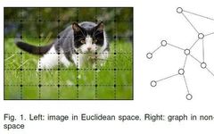
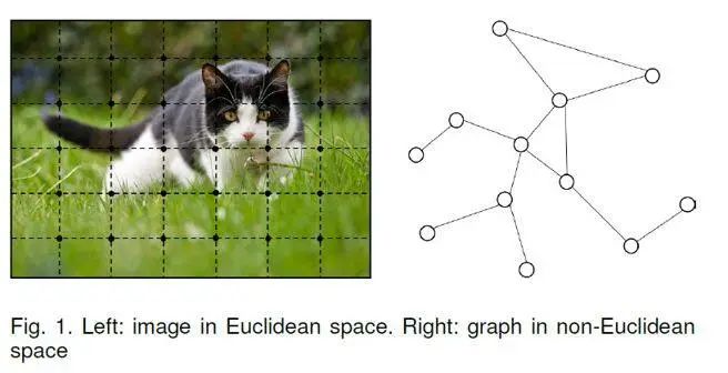
2. The earliest GNNs mainly addressed strict graph theory problems such as molecular structure classification. However, in reality, Euclidean spaces (like images) or sequences (like text) can also be converted into graphs, allowing the application of Graph Neural Network techniques for modeling.

3. After 2009, there were some related studies on Graph Neural Networks, but they did not create much impact. Until 2013, based on Graph Signal Processing, Bruna (a student of LeCun) first proposed convolutional neural networks on graphs based on spectral-domain and spatial-domain in literature.

4. Since then, many spatial-based graph convolution methods have been proposed in academia, and many scholars have attempted to unify previous works within a common framework. However, works based on the frequency domain are relatively few and have only attracted the interest of some scholars.

5. It is worth mentioning that the development history of Graph Neural Networks and Graph Representation Learning is surprisingly similar. In 2014, inspired by word2vec, Perozzi et al. proposed DeepWalk, opening the door to deep learning-era graph representation learning. Interestingly, around the same time, Bordes et al. proposed the famous TransE, laying the foundation for distributed representation in knowledge graphs.

Graph Neural Network (GNN)

First, it should be clarified that unless otherwise specified, the graphs mentioned in this article refer to the graphs in graph theory. It is a type of structure composed of several nodes and edges connecting two nodes, used to depict the relationships between different nodes. Below is a vivid example, the image is from the paper:

>> State Update and Output <<

The earliest Graph Neural Networks originated from Dr. Franco’s paper, and its theoretical foundation is fixed-point theory. Given a graph, each node has its own features, denoted as for the feature of node v; the edges connecting two nodes also have their own features, denoted as for the feature of the edge between node v and node u; The learning objective of GNN is to obtain the graph-aware hidden state (state embedding), which means: for each node, its hidden state contains information from neighboring nodes. So, how does each node perceive other nodes in the graph? GNN achieves this by iteratively updating the hidden states of all nodes, at time t, the hidden state of node is updated as follows:

In the above formula, is the state update function for the hidden state, which is also referred to as the local transaction function in the paper. The in the formula refers to the features of the edges adjacent to node, the refers to the features of the neighboring nodes of node, and refers to the hidden states of neighboring nodes at time t. Note that is applicable to all nodes, and is a globally shared function. So how do we integrate it with deep learning? Smart readers should have thought of using neural networks to fit this complex function. It is worth mentioning that although it seems that the input of is of variable length, we can first transform the variable-length parameters into fixed parameters through certain operations, such as using the sum of all hidden states to represent all hidden states. Let’s illustrate with an example:

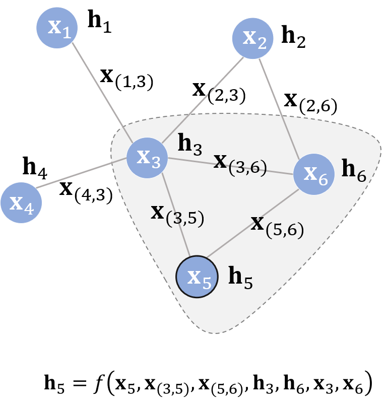
Assuming node is the central node, its hidden state update function is shown in the figure. The idea expressed by this update formula is natural and fitting: continuously using the hidden states of neighboring nodes at the current time as part of the input to generate the hidden state of the central node at the next time, until the changes in the hidden states of each node are minimal, and the information flow of the entire graph stabilizes. At this point, each node is “aware” of the information of its neighbors. The state update formula only describes how to obtain the hidden state of each node; in addition to it, we also need another function to describe how to adapt to downstream tasks. For example, given a social network, a possible downstream task is to determine whether each node is a bot account.

In the original paper, is also called the local output function, which can similarly be expressed by a neural network, and it is also a globally shared function. Thus, the entire process can be expressed in the following diagram:

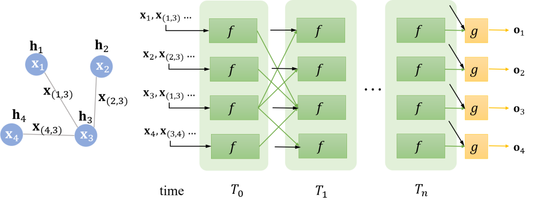
Carefully observe the connections between two time points; they are closely related to the connections in the graph. For example, at time t, the state of node 1 receives the previous hidden state from node 3 because node 1 is adjacent to node 3. Until time t+1, the hidden states of each node converge, and each node followed by a can obtain the output of that node.

For different graphs, the convergence time may vary, as convergence is determined by whether the difference in the -norm between two time points is less than a certain threshold, for example:

>> Example: Compound Classification <<

Now let us give an example to illustrate how Graph Neural Networks are applied in practical scenarios, this example comes from paper [2]. Suppose we now have a task, given the molecular structure of an aromatic compound (including atom types, atomic bonds, etc.), the model’s learning objective is to determine whether it is harmful. This is a typical binary classification problem, and a training sample is as follows:

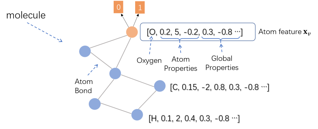
Since the classification of compounds actually requires classifying the entire graph, in the paper, the authors use the representation of the root node of the compound as the representation of the entire graph, as shown by the red node in the figure. Atom features include the type of each atom (Oxygen, oxygen atom), the properties of the atom itself (Atom Properties), some characteristics of the compound (Global Properties), etc. Treating each atom as a node in the graph and atomic bonds as edges, a molecule can be viewed as a graph. After continuously iterating to obtain the converged hidden state of the root node (the oxygen atom), a feedforward neural network can be placed on top as the output layer (i.e., the function) to perform binary classification on the entire compound.

Of course, in homogeneous graphs, selecting the same root node based on the strategy is also very important. However, we will not focus on this part of the details here; interested readers can refer to the original text.

Fixed-point Theory At the beginning of this section, we mentioned that the theoretical basis of GNN is fixed-point theory, which specifically refers to Banach’s Fixed Point Theorem. First, we denote the function obtained by stacking several as the global update function, then the state update formula for all nodes on the graph can be written as:

The fixed-point theorem states that regardless of what is, as long as is a contraction map, it will converge to a fixed point through continuous iterations, which we call the fixed point. So what is a contraction map? A graph can explain it clearly:

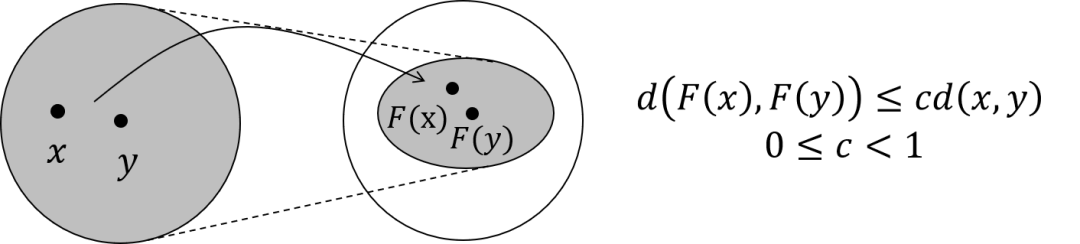
The solid arrows in the figure indicate the mapping , and any two points will be transformed into after passing through this mapping. A contraction map means that, after transformation, the new space is definitely smaller than the original space, meaning the original space has been compressed. Imagine this compression process occurring continuously, eventually mapping all points in the original space to a single point.

Then, some readers may wonder, since is implemented by a neural network, how can we ensure that it is a contraction map? Let’s talk about the specific implementation of .

Specific Implementation In the specific implementation, can actually be realized through a simple feedforward neural network. For example, one implementation method could be to simply concatenate the features of each neighboring node, the hidden state, the features of each connected edge, and the features of the node itself, and after passing through a feedforward neural network, perform a simple summation.

So how do we ensure that is a contraction map? It is actually achieved by restricting the size of the Jacobian matrix of with respect to , which is implemented through a penalty term on the Jacobian matrix. In algebra, there is a theorem stating that the equivalent condition for to be a contraction map is that the gradient/derivative of should be less than 1. This equivalent theorem can be derived from the formal definition of contraction mapping, and here we use to denote the norm of in space.

Norm is a scalar, representing the length or magnitude of a vector, and is a continuous function of coordinates in finite space. Here we simplify it to one dimension, where the difference between coordinates can be viewed as the distance between vectors in space. Based on the definition of contraction mapping, we can derive:

To generalize, we get that the penalty term for the Jacobian matrix needs to satisfy its norm being less than or equal to the equivalent condition of contraction mapping. According to the Lagrange multiplier method, we can transform the constrained problem into an unconstrained optimization problem with a penalty term, and the training objective can be represented in the following form:

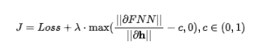
where is a hyperparameter, and the term multiplied by it is the penalty term of the Jacobian matrix.

>> Model Learning <<

Above, we spent some space to understand how to make approach a contraction map; now let’s specifically describe how the loss of the Graph Neural Network is defined and how the model learns.

Still taking social networks as an example, although each node will have a hidden state and an output, not every node will have a supervision signal. For example, in a social network, only some users are explicitly labeled as bot accounts, forming a typical node binary classification problem.

So naturally, the model’s loss is obtained through these supervised nodes. Suppose there are a total of supervised nodes, the model loss can be formalized as:

So how does the model learn? Based on the forward propagation process for calculating the loss, it is not difficult to derive the backward propagation process for calculating the gradient. In forward propagation, the model:

calls several times, for example, times, until converges. At this point, the hidden states of each node approach the solution of the fixed point. For the nodes with supervision signals, their hidden states are processed through to obtain the output, and thus the model’s loss is calculated. According to the above process, during backward propagation, we can directly calculate the gradient of and with respect to the final hidden state . However, because the model recursively calls several times, to calculate the gradient of and with respect to the initial hidden state , we need to recursively/iteratively calculate the gradient of times as well. The final obtained gradient will be the gradient of and with respect to , and this gradient is then used to update the model parameters. This algorithm is known as the Almeida-Pineda algorithm.

>> GNN and RNN <<

Those familiar with RNN/LSTM/GRU and other recurrent neural networks may feel a bit confused at this point because Graph Neural Networks, both in terms of forward propagation and the optimization algorithm for backward propagation, are somewhat similar to recurrent neural networks. This is not your illusion; in fact, Graph Neural Networks are indeed quite similar to recurrent neural networks. To clearly show the differences between them, we can use a diagram to explain the design differences:

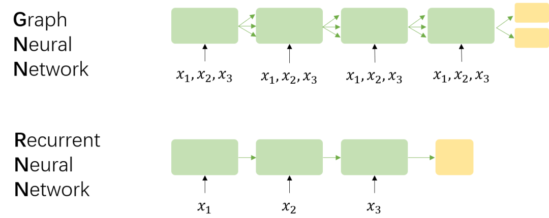
Assuming there are three nodes ,, in GNN, correspondingly, there is a sequence in RNN. I believe the differences between GNN and RNN mainly lie in four points:

1. The foundational theory of GNN is fixed-point theory, which means the length of GNN’s temporal unfolding is dynamic and determined by convergence conditions, while the length of RNN’s temporal unfolding is equal to the length of the sequence itself.

2. In GNN, the input at each time step is the features of all nodes , while in RNN, the input at each time step is the input corresponding to that time step. Meanwhile, the flow of information between time steps is also different; the former is determined by edges, while the latter is determined by the order of sequence input.

3. GNN uses the AP algorithm for backward propagation optimization, while RNN uses BPTT (Back Propagation Through Time) optimization. The former requires convergence, while the latter does not.

4. The goal of GNN’s recursive call of is to obtain stable hidden states for each node, so outputs can only be generated after the hidden states converge; while RNN can output at each time step, such as in language models.

However, given the structural similarity between the initial GNN and RNN, some articles also like to refer to it as Recurrent-based GNN, and some articles classify it under Recurrent-based GCN. Readers will understand why people name it this way after learning about GCN.

>> Limitations of GNN <<

The initial GNN, which is based on a recurrent structure, has its core in fixed-point theory. Its main idea is to achieve convergence of the entire graph through the propagation of node information, and then make predictions based on that. Convergence, being the core of GNN, also limits its broader usage, with two prominent issues:

1. GNN treats edges merely as a means of propagation, but does not distinguish the functions of different edges. Although we can assign different features to different types of edges during the feature construction stage, compared to other inputs, the influence of edges on the hidden states of nodes is indeed limited. Moreover, GNN does not set independent learnable parameters for edges, meaning it cannot learn certain characteristics of edges through the model.

2. If GNN is applied in graph representation scenarios, using fixed-point theory is not appropriate. This is mainly because the convergence based on fixed points will lead to excessive information sharing among the hidden states of nodes, resulting in the hidden states of nodes becoming overly smooth (Over Smooth), and the feature information belonging to the nodes themselves becoming scarce (Less Informative).

The following image from Wikipedia can vividly explain what Over Smooth is. Here, we consider the entire layout as a graph, where each pixel is adjacent to its 8 neighboring pixels. This determines the path of information flow on the graph. Initially, blue represents no information, which can be expressed as an empty vector; green, yellow, and red each have some information, expressed as non-empty feature vectors. On the graph, information mainly flows from three areas with distinct features to their adjacent pixels. At first, the distinction between different pixels is very clear, but during the transition to a fixed point, all pixels become uniform, resulting in a homogeneous distribution. Thus, although each pixel perceives global information, we cannot distinguish them based on their final hidden states. For example, based on the final states, we cannot tell which pixels were initially in the green area.

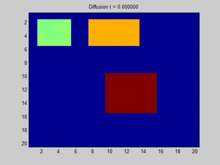
Here, I would like to elaborate a bit more. In fact, the above image is not entirely equivalent to the information flow in GNN. From my perspective, if we use a physical model to describe it, the above image represents three heat sources initially radiating heat, and then allowing them to evolve freely; however, in reality, GNN updates the hidden states of nodes at each time step by taking the features as inputs, as if several everlasting heat sources were placed, and the heat sources would interfere with each other but ultimately would not become completely identical.

Gated Graph Neural Network (GGNN)

We have meticulously compared GNN and RNN, and we can see that they share many similarities. So, can we directly define GNN using a method similar to RNN? Thus, the Gated Graph Neural Network (GGNN) appeared. Although they may seem similar here, their differences are significant, with the most core difference being that gated neural networks are not based on fixed-point theory. This means: it is no longer necessary for it to be a contraction map; iterations do not need to converge to output; and the optimization algorithm also shifts from the AP algorithm to BPTT.

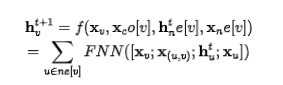
State Update and the paradigm defined by Graph Neural Networks are consistent; GGNN also has two processes: state update and output. Compared to GNN, its main difference arises from the state update stage. Specifically, GGNN refers to the design of GRU, treating the information of neighboring nodes as input and the state of the node itself as hidden state, its state update function is as follows:

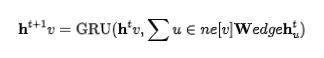
If the reader is familiar with the update formula of GRU, they should find the above formula easy to understand. Notably, apart from the GRU-style design, GGNN also introduces learnable parameters for different types of edges, each corresponding to a , allowing it to handle heterogeneous graphs.

However, upon careful comparison of GGNN’s state update formula with that of GNN, attentive readers may notice that the node features required as inputs in GNN do not appear in GGNN’s formula! But in reality, these node features are crucial for our predictions, as they are fundamental to each node.

To address this issue, GGNN incorporates node features as part of the initialization of hidden states. So, to revisit GGNN’s process, it actually goes like this:

1. Initialize the (partial) hidden states of each node with node features;

2. For the entire graph, iteratively apply the state update formula for a fixed number of times;

3. Calculate the model loss for nodes with supervised signals and use the BPTT algorithm for backpropagation to obtain the gradients of and GRU parameters.

Example 1: Reachability Judgment To facilitate understanding, we provide an example from paper [10]. Suppose we are given a graph, starting node , and for any node , the model judges whether the starting node can walk through the graph to reach that node. Similarly, this can be transformed into a binary classification problem for nodes, i.e., reachable and not reachable. The following figure describes such a process:

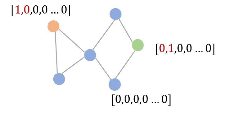
The red node in the figure is the starting node, and the green node is the one we wish to judge, referred to as the ending node. Compared to other nodes, these two nodes have certain uniqueness. We can represent the starting node with a 1 in the first dimension and the ending node with a 1 in the second dimension. Finally, when classifying the ending node, if its hidden state’s first dimension is assigned a non-zero real value, it means it can be reached.

From the initialization process, we can also see the differences between GNN and GGNN: GNN relies on fixed-point theory, so even with random initialization, each node’s hidden state will converge to a fixed point; GGNN, on the other hand, is different, as different initializations significantly impact GGNN’s final results.

Example 2: Semantic Parsing The above example illustrates the differences between GNN and GGNN very simply and vividly. As I am particularly interested in work related to Semantic Parsing, I will borrow a paper from ACL 2019 [11] to discuss how GGNN is used in practice and the scenarios it is suitable for.

First, let me provide some background for readers unfamiliar with semantic parsing. The main task of semantic parsing is to convert natural language into machine language, specifically referring to SQL (Structured Query Language), which is the well-known database query language. What is the use of this task? It allows novice users to obtain the data they care about from databases without having to learn SQL syntax or have programming foundations, enabling direct database queries through natural language. In fact, semantic parsing remains a very challenging task today. Apart from the semantic expression gap between natural language and programming language, a significant portion of performance loss is due to the complexity of the task itself, or the syntax of SQL language. For example, we have two tables, one recording student IDs and their genders, and the other recording the courses each student has enrolled in. To find out how many female students have enrolled in a particular course, we need to join the two tables, filter the results, and perform aggregate statistics. This issue is particularly prominent in multi-table scenarios, where each table is interconnected through foreign keys. In fact, if we treat the headers in the tables as nodes, and the connections between nodes as edges, we can form a graph, as illustrated in the middle of the figure below:

Paper [11] utilizes this table feature and employs GGNN to solve multi-table problems. We will first introduce a general semantic parsing method, and then discuss how [11] connects graphs with semantic parsing systems. As far as I know, the vast majority of semantic parsing methods currently follow a Seq2seq framework, where the input consists of individual natural language words and the output consists of individual SQL words. However, this framework does not consider the implicit constraints that tables impose on SQL outputs. For instance, in a single SELECT clause, the headers we select must come from the same table. Another example is that two tables that can be JOINed must have a foreign key relationship, just like the example we mentioned about students enrolling in courses.

So, how can GGNN be integrated into traditional semantic parsing methods? In paper [11], this is accomplished through three steps:

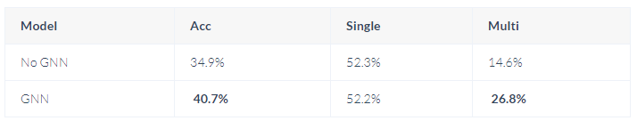
First, establish the corresponding graph based on the table. Then, utilize GGNN to compute the hidden states of each header. Finally, during the encoding phase of the Seq2seq model, use the word vectors of each input natural language word to compute an attention score for all header hidden states of the table, obtaining a graph-aware representation for each natural language word based on the attention weights. In the decoding phase, if the output is a word like header/table from the table, the output vector is scored against the hidden states of all headers/tables in the table, which is provided by . In fact, this is a fully connected layer, and its output represents the degree of correlation between SQL words and each header/table in the table. To ensure that each output of SQL is consistent with historical information, each time an output is made, previously outputted headers/tables are used to score the candidates in the header/table, thus utilizing multi-table information. The performance of this paper on multi-table tasks is indeed very good, and below is a performance comparison on the Spider dataset:

GNN and GGNN GGNN has currently received widespread application; compared to GNN, its biggest difference is that it is no longer based on fixed-point theory. Although this means that convergence is no longer required, it also means that GGNN’s initialization is crucial. From the literature I have read, most of the work following GNN has shifted towards aligning GNN with traditional RNN/CNN, which potentially allows for continuous absorption of improvements from these two research areas. However, there are very few works based on the original GNN grounded in fixed-point theory; at least during my literature review, I did not find much related work.

But from another perspective, although GNN and GGNN have different theories, their design philosophy is remarkably similar to that of recurrent neural networks.

1. The advantage of recurrent neural networks lies in their ability to handle sequences of arbitrary length, but their computation must be serially processed over several time steps, which incurs non-negligible time costs. Therefore, the two recurrent-based Graph Neural Networks are not very efficient when updating hidden states. If we draw on the successful experience of stacking multiple layers in deep learning, we have sufficient reason to believe that multi-layer Graph Neural Networks can achieve similar effects.

2. Recurrent-based Graph Neural Networks share the same parameters at each iteration, while multi-layer neural networks have different parameters at each layer, which can be viewed as a method of hierarchical feature extraction.

Original address:https://www.cnblogs.com/SivilTaram/p/graph_neural_network_1.htmlReferences [1]. A Comprehensive Survey on Graph Neural Networks, https://arxiv.org/abs/1901.00596[2]. The graph neural network model, https://persagen.com/files/misc/scarselli2009graph.pdf[3]. Spectral networks and locally connected networks on graphs, https://arxiv.org/abs/1312.6203[4]. Distributed Representations of Words and Phrases and their Compositionality, http://papers.nips.cc/paper/5021-distributed-representations-of-words-andphrases[5]. DeepWalk: Online Learning of Social Representations, https://arxiv.org/abs/1403.6652[6]. Translating Embeddings for Modeling Multi-relational Data, https://papers.nips.cc/paper/5071-translating-embeddings-for-modeling-multi-relational-data[7]. Deep Learning on Graphs: A Survey, https://arxiv.org/abs/1812.04202[8]. How to understand Graph Convolutional Network (GCN)? https://www.zhihu.com/question/54504471[9]. Almeida–Pineda recurrent backpropagation, https://www.wikiwand.com/en/Almeida%E2%80%93Pineda_recurrent_backpropagation[10]. Gated graph sequence neural networks, https://arxiv.org/abs/1511.05493[11]. Representing Schema Structure with Graph Neural Networks for Text-to-SQL Parsing, https://arxiv.org/abs/1905.06241[12]. Spider1.0 Yale Semantic Parsing and Text-to-SQL Challenge, https://yale-lily.github.io/spider[13]. https://www.wikiwand.com/en/Laplacian_matrix