An Analysis of word2vec Source Code

word2vec was launched by Google in 2013. The methods for obtaining word vectors, CBOW and Skip-gram models, are elaborated in the paper “Efficient Estimation of Word Representations in Vector Space.” The strategies for efficiently training models, Hierarchical Softmax and Negative Sampling, are discussed in “Distributed Representations of Words and Phrases and their Compositionality.” Since the two papers published by Mikolov are not easy to understand, you can refer to Xin Rong’s “word2vec parameter learning explained,” or directly look at the article published by peghoty on his blog, “Detailed Explanation of Mathematical Principles in word2vec.” There are numerous articles about word2vec online, but they mainly relate to its mathematical principles. This article focuses on reading and analyzing the source code open-sourced by Mikolov on GitHub, and also references others’ blogs and the Python version (if you are familiar with Python, it is recommended to look at this version, as it feels clearer). This part will be listed at the end of the article.
The source code of word2vec involves a large number of file read operations, building vocabulary and hash tables, as well as corresponding queries, comparisons, sorting, and other auxiliary functions. This part will not be analyzed in detail in this article; instead, we will focus on the implementations of Hierarchical Softmax, Negative Sampling, Skip-gram, and CBOW.
I generally start reading the source code from the main function, as this section contains the entire code execution process. Starting from the main function, I then read the classes and methods involved in each step. The code related to training in word2vec is in TrainModel. I believe the key points here are: the network initialization parameter module and the training module. The former includes InitNet, CreateBinaryTree, and InitUnigramTable, while the latter corresponds to the TrainModelThread in the code, mainly for CBOW and Skip-gram. Below, I will analyze these two parts separately.

01

Network Initialization Parameters

This section mainly involves the construction of the Huffman tree and UnigramTable, which are the foundational work for the subsequent Hierarchical Softmax and Negative Sampling.

1. InitNet

This part mainly initializes a projection layer’s network structure, where vocab_size is the length of the vocabulary, and layer1_size is the length of the output word vector. If Hierarchical Softmax is used, i.e., hs=1, it will initialize an auxiliary vector syn1 of size vocab_size*layer1_size filled with zeros, used to store the non-leaf nodes in the constructed Huffman tree.
If Negative Sampling is used, it will initialize an auxiliary vector syn1neg of size vocab_size*layer1_size filled with zeros. Syn0 is the word vector we ultimately need, initialized as a random vector of size vocab_size*layer1_size within the interval [-0.5/layer1_size, 0.5/layer1_size].
The specific code is as follows:
void InitNet() {  long long a, b;  unsigned long long next_random = 1;  a = posix_memalign((void **)&syn0, 128, (long long)vocab_size * layer1_size * sizeof(real));  if (syn0 == NULL) {printf("Memory allocation failed\n"); exit(1);}  if (hs) {    a = posix_memalign((void **)&syn1, 128, (long long)vocab_size * layer1_size * sizeof(real));    if (syn1 == NULL) {printf("Memory allocation failed\n"); exit(1);}    for (a = 0; a < vocab_size; a++) for (b = 0; b < layer1_size; b++)     syn1[a * layer1_size + b] = 0;  }  if (negative>0) {    a = posix_memalign((void **)&syn1neg, 128, (long long)vocab_size * layer1_size * sizeof(real));    if (syn1neg == NULL) {printf("Memory allocation failed\n"); exit(1);}    for (a = 0; a < vocab_size; a++) for (b = 0; b < layer1_size; b++)     syn1neg[a * layer1_size + b] = 0;  }  for (a = 0; a < vocab_size; a++) for (b = 0; b < layer1_size; b++) {    next_random = next_random * (unsigned long long)25214903917 + 11;    syn0[a * layer1_size + b] = (((next_random & 0xFFFF) / (real)65536) - 0.5) / layer1_size;  }}

2. CreateBinaryTree

This part creates the Huffman binary tree, which mainly provides the corresponding data structure foundation for the implementation of the Hierarchical Softmax method.
The pseudocode for building the Huffman tree is as follows:
Input: n nodes with weights (𝑀1,𝑀2,…𝑀𝑛)
Output: Corresponding Huffman tree
1) Treat (𝑀1,𝑀2,…𝑀𝑛) as a forest with n trees, each with only one node.;
2) Select the two trees with the smallest root node weights from the forest to merge, resulting in a new tree, where these two trees become the left and right subtrees of the new tree. The weight of the new tree’s root node is the sum of the weights of the root nodes of the left and right subtrees;
3) Remove the two trees with the smallest root node weights from the forest and add the new tree to the forest;
4) Repeat steps 2) and 3) until there is only one tree left in the forest.
According to the characteristics of the Huffman tree, the higher the weight of a word, the shorter the path on the binary tree, meaning the binary encoding is shorter and closer to the root node. This aligns with our business understanding that more commonly used words have shorter encodings. The code for creating the Huffman tree in word2vec is as follows.
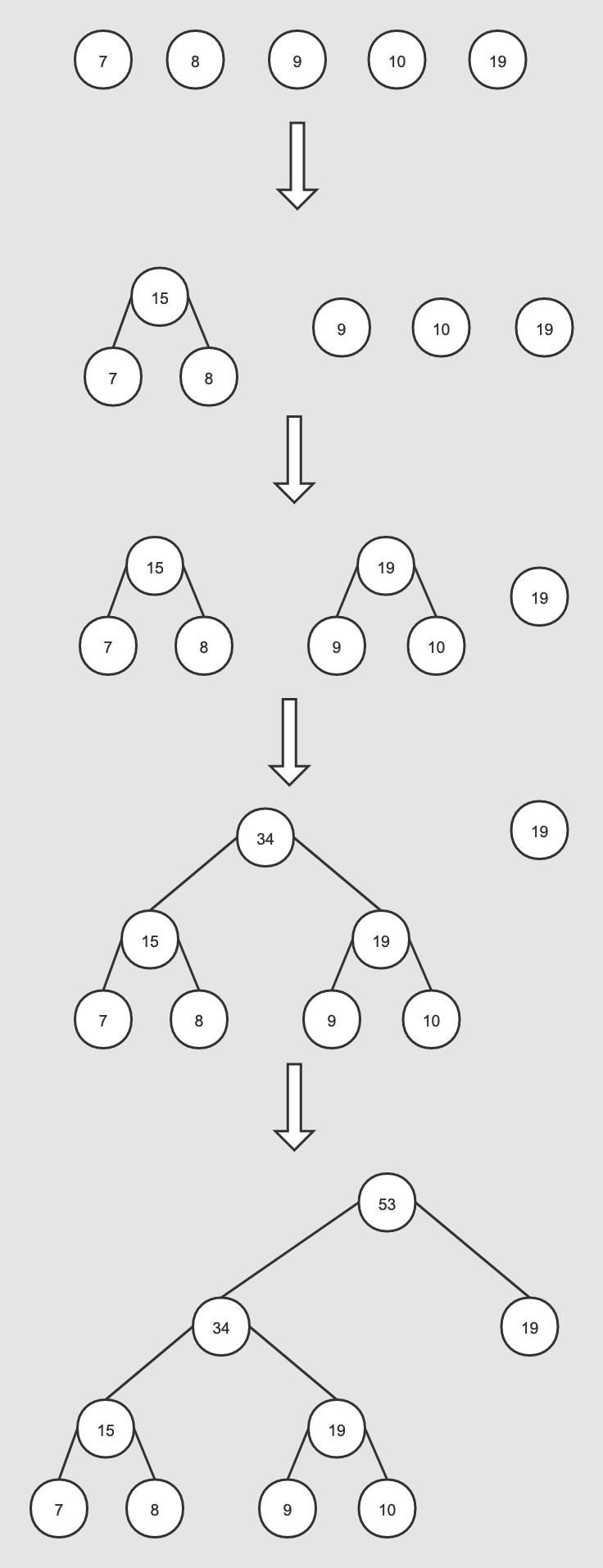
void CreateBinaryTree() {  long long a, b, i, min1i, min2i, pos1, pos2, point[MAX_CODE_LENGTH];  char code[MAX_CODE_LENGTH];  long long *count = (long long *)calloc(vocab_size * 2 + 1, sizeof(long long));  long long *binary = (long long *)calloc(vocab_size * 2 + 1, sizeof(long long));  long long *parent_node = (long long *)calloc(vocab_size * 2 + 1, sizeof(long long));  for (a = 0; a < vocab_size; a++) count[a] = vocab[a].cn;  for (a = vocab_size; a < vocab_size * 2; a++) count[a] = 1e15;  pos1 = vocab_size - 1;  pos2 = vocab_size;  for (a = 0; a < vocab_size - 1; a++) {    if (pos1 >= 0) {      if (count[pos1] < count[pos2]) {        min1i = pos1;        pos1--;      } else {        min1i = pos2;        pos2++;      }    } else {      min1i = pos2;      pos2++;    }    if (pos1 >= 0) {      if (count[pos1] < count[pos2]) {        min2i = pos1;        pos1--;      } else {        min2i = pos2;        pos2++;      }    } else {      min2i = pos2;      pos2++;    }    count[vocab_size + a] = count[min1i] + count[min2i];    parent_node[min1i] = vocab_size + a;    parent_node[min2i] = vocab_size + a;    binary[min2i] = 1;  }  for (a = 0; a < vocab_size; a++) {    b = a;    i = 0;    while (1) {      code[i] = binary[b];      point[i] = b;      i++;      b = parent_node[b];      if (b == vocab_size * 2 - 2) break;    }    vocab[a].codelen = i;    vocab[a].point[0] = vocab_size - 2;    for (b = 0; b < i; b++) {      vocab[a].code[i - b - 1] = code[b];      vocab[a].point[i - b] = point[b] - vocab_size;    }  }  free(count);  free(binary);  free(parent_node);}
First, we need to define point and code, where point is used to store the path from a word to the root node of the Huffman tree, and code is used to store the Huffman encoding of a word. The code also defines count, binary, and parent_node arrays, all of length vocab_size*2+1, where the first vocab_size of the count array represents the leaf nodes of the Huffman tree, initialized with the word frequencies of all words in the vocabulary, and the latter vocab_size represents the frequencies of the non-leaf nodes that are about to be generated in the Huffman tree, initialized to 1e15 through the merging of child nodes’ weights. The binary array records the binary encoding of each node relative to its parent node, and parent_node records each node’s parent node.
Next is to build the Huffman tree. Note that the input count array’s first vocab_size has been sorted in descending order by word frequency. The initial pos1 and pos2 are the indices of the words with the lowest frequencies in the vocabulary and the first 1e15, respectively. Later, by comparing the current pos1 and pos2’s corresponding word frequencies, we update the indices min1i and min2i of the current minimum and second minimum frequencies.
Taking the original sequence {‘u’: 7, ‘v’: 8, ‘w’: 9, ‘x’: 10, ‘y’: 19} as an example, the initial word frequencies are [19, 10, 9, 8, 7], and the corresponding count array is [19, 10, 9, 8, 7, 1e15, 1e15, 1e15, 1e15, 1e15].
  • In the first iteration, a=0, pos1=4, pos2=5, count[pos1]=7, count[pos2]=1e15. At this point, count[pos1] < count[pos2], so min1i=4, pos1 decreases to 3, count[pos1]=8, count[pos2]=1e15, count[pos1] < count[pos2], min2i=3, pos1 decreases to 2, count[5+0] is assigned count[3]+count[4]=15.

  • In the second iteration, a=1, pos1=2, pos2=5, count[pos1]=9, count[pos2]=15. At this point, count[pos1] < count[pos2], so min1i=2, pos1 decreases to 1, count[pos1]=10, count[pos2]=1e15, count[pos1] < count[pos2], min2i=1, pos1 decreases to 0, count[5+1] is assigned count[1]+count[2]=19.

  • In the third iteration, a=2, pos1=0, pos2=5, count[pos1]=19, count[pos2]=15. At this point, count[pos1] > count[pos2], so min1i=5, pos2 increases to 6, count[pos1]=19, count[pos2]=19, count[pos1] = count[pos2], min2i=6, pos2 increases to 7, count[5+2] is assigned count[5]+count[6]=34.

  • In the fourth iteration, a=3, pos1=0, pos2=7, count[pos1]=19, count[pos2]=34. At this point, count[pos1] < count[pos2], so min1i=0, pos1 decreases to -1, at this point, pos1 is less than 0, min2i=7, pos2 increases to 8, count[5+3] is assigned count[0]+count[7]=53.

An Analysis of word2vec Source Code

Since we are constructing a Huffman tree, at most, we only need to perform vocab_size-1 loop operations. The entire iteration process is to obtain the smallest count[min1i] and second smallest count[min2i], merge (sum), and then repeat this step until the iteration ends. In each iteration, the binary array’s index min2i will be set to 1, meaning the lower frequency is 1, and the higher frequency is 0. The parent_node will set the elements indexed by min1i and min2i in each iteration to a+vocab_size.
Next, we traverse all the words in the vocabulary and assign each word its path and encoding in the Huffman tree. It is important to note:
  • Establish a temporary variable b, mainly to obtain the current word’s path in parent_node, which also directly corresponds to the index in binary;

  • Since the Huffman tree has a total of vocab_size*2-1 nodes, vocab_size*2-2 is the root node. The code uses this as the termination condition for the loop, meaning the path has reached the root node;

  • Since the Huffman encoding and path go from the root node to the leaf node, we need to reverse the previously obtained code and point, and the path should also have vocab_size subtracted.

Taking the word ‘w’ from the above sequence as an example, with a frequency of 9 and an index of 2, i.e., a=2, the previous binary sequence is [0, 1, 0, 1, 0, 0, 1, 1, 0, 0, 0], and parent_node is [8, 6, 6, 5, 5, 7, 7, 8, 0, 0, 0]. The resulting code for ‘w’ is [0, 1, 1], and point=[2, 6, 7]. Since the Huffman path stores the intermediate node numbers, we need to subtract vocab_size from the newly obtained base, meaning not counting the leaf nodes, and only taking the pure intermediate node numbers. Therefore, the root node number is (vocab_size*2-2) – vocab_size = vocab_size – 2, which in this example is 3. After reversing, vocab[2].code is [1, 1, 0], and vocab[2].point is [3, 2, 1, -3].
At this point, the Huffman encoding and path corresponding to each word have been calculated.

3. InitUnigramTable

Construct a power law distribution table for each word in the vocabulary for subsequent negative sampling. Taking the 0.75 power of the word frequency is actually a smoothing strategy, reducing the frequency gap between words. The specific code is as follows.
void InitUnigramTable() {  int a, i;  double train_words_pow = 0;  double d1, power = 0.75;  table = (int *)malloc(table_size * sizeof(int));  for (a = 0; a < vocab_size; a++) train_words_pow += pow(vocab[a].cn, power);  i = 0;  d1 = pow(vocab[i].cn, power) / train_words_pow;  for (a = 0; a < table_size; a++) {    table[a] = i;    if (a / (double)table_size > d1) {      i++;      d1 += pow(vocab[i].cn, power) / train_words_pow;    }    if (i >= vocab_size) i = vocab_size - 1;  }}
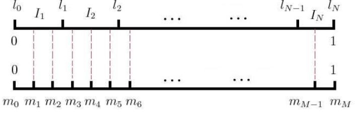
The initialized table_size is 1e8. Then, traverse the vocabulary; train_words_pow is the cumulative sum of each word’s frequency cn^0.75. Next, calculate the ratio of a single word to train_words_pow, d1. If a/table_size does not exceed the current word’s d1, i will not increment, meaning the current word will occupy a+n-a positions. Otherwise, d1’s value will be cumulatively updated. The reason for the accumulation is that there is no need to compare from the beginning; the position a continues to move forward, and the corresponding d1 should also accumulate based on the previous basis, maintaining the relative position unchanged while updating the absolute position. Thus, each word will correspond to a segment, and words in the same segment are the same, so when sampling, just specify neg index positions, and it will inevitably take neg words.
An Analysis of word2vec Source Code
If the vocabulary length is smaller than the UnigramTable, that is, if the UnigramTable is not filled, fill the unfilled part with the last word in the vocabulary.

02

Training Module

Whether it is CBOW or Skip-gram, the code uses the following variables, which I will introduce first:
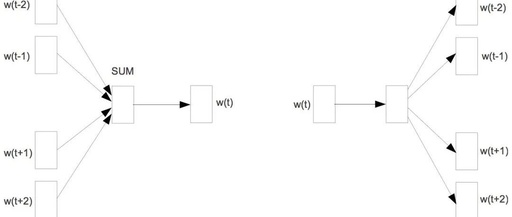
  • neu1: Input word vector [in CBOW, it is the sum of the vectors of words in the window; in Skip-gram, it is the vector of the center word], length is layer1_size, initialized to 0, used to update syn1;

  • neu1e: Length is layer1_size, initialized to 0, used to update syn0;

  • alpha: Learning rate;

  • last_word: Records the index of the current context word being scanned.
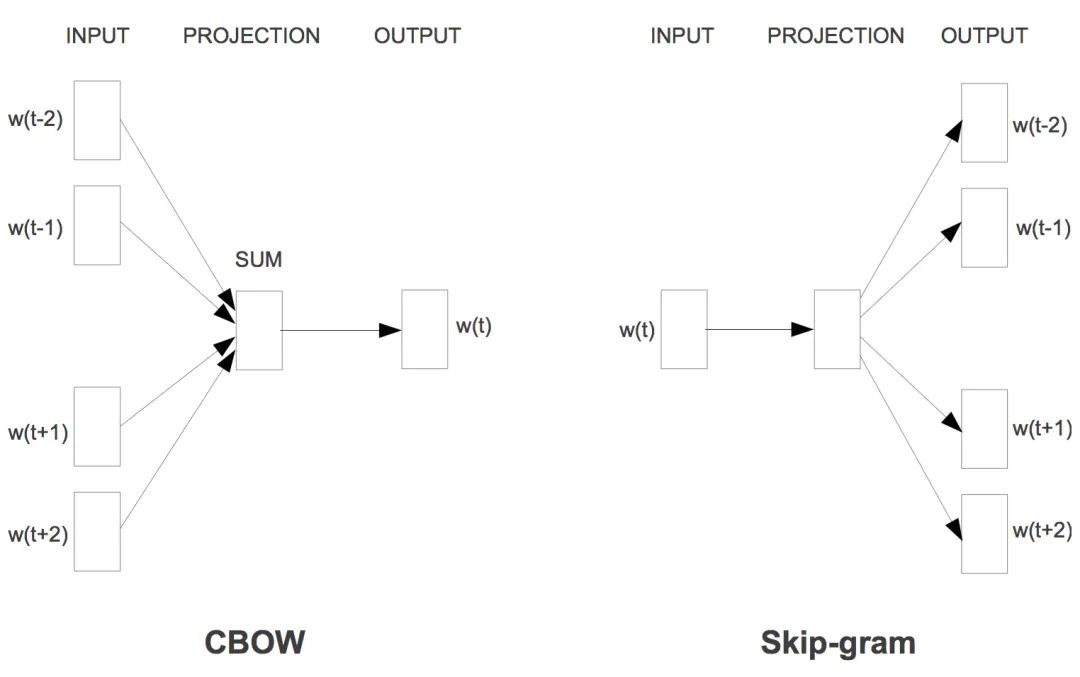
An Analysis of word2vec Source Code

1. CBOW

CBOW requires us to predict the center word based on the context window words. Here, we first calculate the sum of the window word vectors and average them. cw is the window length, establishing the association between the center word and the window words.
for (c = 0; c < layer1_size; c++) neu1[c] += syn0[c + last_word * layer1_size];for (c = 0; c < layer1_size; c++) neu1[c] /= cw;

1.1 Training Using Hierarchical Softmax

According to the previously constructed Huffman tree, traverse all intermediate nodes passed from the root node to the current word’s leaf node. l2 is the position of the current intermediate node vector in syn1, and f is the accumulation of neu1 at l2 within layer1_size range. Essentially, this is the inner product of neu1 and the intermediate node vector. Here, codelen is the tree depth, and during the loop, we can directly filter out the -3 corresponding to the example ‘w’ in the point.
Next, we perform a Sigmoid transformation on f. Here, we maintain an expTable array, allowing us to directly look up the transformation result by index. Then, we calculate the error between f and the Huffman encoding of each word obtained earlier and perform gradient updates. It is important to note that the nodes with encoding 1 will be defined as negative classes, while 0 is positive, meaning the true label is 1-vocab[word].code[d]. Finally, we update the vectors at the corresponding positions of neu1e and syn1, where each iteration is a logistic regression, and the whole process is essentially a maximization of the log-likelihood function using stochastic gradient ascent.
for (d = 0; d < vocab[word].codelen; d++) {      f = 0;      l2 = vocab[word].point[d] * layer1_size;      for (c = 0; c < layer1_size; c++) f += neu1[c] * syn1[c + l2];      if (f <= -MAX_EXP) continue;      else if (f >= MAX_EXP) continue;      else f = expTable[(int)((f + MAX_EXP) * (EXP_TABLE_SIZE / MAX_EXP / 2))];      g = (1 - vocab[word].code[d] - f) * alpha;      for (c = 0; c < layer1_size; c++) neu1e[c] += g * syn1[c + l2];      for (c = 0; c < layer1_size; c++) syn1[c + l2] += g * neu1[c];    }

1.2 Training Using Negative Sampling

In this case, negative is the number of negative samples. When d=0, we obtain the target word and designate it as a positive sample. Otherwise, we randomly select negative samples from the UnigramTable (which cannot be the same as the current positive sample). Here, l2 is the position of the target word in syn1neg, and the rest is basically the same as Hierarchical Softmax, so I won’t elaborate further.
for (d = 0; d < negative + 1; d++) {      if (d == 0) {        target = word;        label = 1;      } else {        next_random = next_random * (unsigned long long)25214903917 + 11;        target = table[(next_random >> 16) % table_size];        if (target == 0) target = next_random % (vocab_size - 1) + 1;        if (target == word) continue;        label = 0;      }      l2 = target * layer1_size;      f = 0;      for (c = 0; c < layer1_size; c++) f += neu1[c] * syn1neg[c + l2];      if (f > MAX_EXP) g = (label - 1) * alpha;      else if (f < -MAX_EXP) g = (label - 0) * alpha;      else g = (label - expTable[(int)((f + MAX_EXP) * (EXP_TABLE_SIZE / MAX_EXP / 2))]) * alpha;      for (c = 0; c < layer1_size; c++) neu1e[c] += g * syn1neg[c + l2];      for (c = 0; c < layer1_size; c++) syn1neg[c + l2] += g * neu1[c];    }
Finally, we update syn0 in real-time based on the obtained neu1e, thus obtaining the final trained word vectors of size vocab_size*layer1_size.
for (a = b; a < window * 2 + 1 - b; a++) if (a != window) {        c = sentence_position - window + a;        if (c < 0) continue;        if (c >= sentence_length) continue;        last_word = sen[c];        if (last_word == -1) continue;        for (c = 0; c < layer1_size; c++) syn0[c + last_word * layer1_size] += neu1e[c];      }

2. Skip-gram

Skip-gram requires us to predict the context window words based on the input center word. The last_word in the code is the current context word to be predicted, and l1 is the position of the current word’s vector in syn0, initializing neu1e to 0.
The training part is generally consistent with the previous section. The difference is that instead of using neu1[c] for the inner product with the intermediate node vector, we directly replace it with syn0[c + l1], where syn0[c + l1] is the vector of a single word, while neu1[c] is the average of the window word vectors. Additionally, it should be noted that although Skip-gram is given the center word to predict the context, during training, it still uses the context to predict the center word.
for (a = b; a < window * 2 + 1 - b; a++) if (a != window) {      c = sentence_position - window + a;      if (c < 0) continue;      if (c >= sentence_length) continue;      last_word = sen[c];      if (last_word == -1) continue;      l1 = last_word * layer1_size;      for (c = 0; c < layer1_size; c++) neu1e[c] = 0;        if (hs) for (d = 0; d < vocab[word].codelen; d++) {          f = 0;          l2 = vocab[word].point[d] * layer1_size;          for (c = 0; c < layer1_size; c++) f += syn0[c + l1] * syn1[c + l2];          if (f <= -MAX_EXP) continue;          else if (f >= MAX_EXP) continue;          else f = expTable[(int)((f + MAX_EXP) * (EXP_TABLE_SIZE / MAX_EXP / 2))];          g = (1 - vocab[word].code[d] - f) * alpha;          for (c = 0; c < layer1_size; c++) neu1e[c] += g * syn1[c + l2];          for (c = 0; c < layer1_size; c++) syn1[c + l2] += g * syn0[c + l1];        }        if (negative > 0) for (d = 0; d < negative + 1; d++) {          if (d == 0) {            target = word;            label = 1;          } else {            next_random = next_random * (unsigned long long)25214903917 + 11;            target = table[(next_random >> 16) % table_size];            if (target == 0) target = next_random % (vocab_size - 1) + 1;            if (target == word) continue;            label = 0;          }          l2 = target * layer1_size;          f = 0;          for (c = 0; c < layer1_size; c++) f += syn0[c + l1] * syn1neg[c + l2];          if (f > MAX_EXP) g = (label - 1) * alpha;          else if (f < -MAX_EXP) g = (label - 0) * alpha;          else g = (label - expTable[(int)((f + MAX_EXP) * (EXP_TABLE_SIZE / MAX_EXP / 2))]) * alpha;          for (c = 0; c < layer1_size; c++) neu1e[c] += g * syn1neg[c + l2];          for (c = 0; c < layer1_size; c++) syn1neg[c + l2] += g * syn0[c + l1];        }        for (c = 0; c < layer1_size; c++) syn0[c + l1] += neu1e[c];      }
An Analysis of word2vec Source Code
Other tricks in the code:
  1. When reading files, a “</s>” is added to the end of each line for easier training.

  2. If the vocabulary size exceeds the limit, a vocabulary reduction operation is performed, deleting current words with frequencies less than min_reduce (initially set to 1). This deletion operation is done in a while(1) loop, where min_reduce increments by 1, ensuring that the maximum number of words does not exceed vocab_hash_size * 0.7. The code sets vocab_hash_size = 30000000, meaning the vocabulary can have a maximum of 21 million words. Otherwise, it will keep deleting low-frequency words until this condition is met. The size of expTable is 1e8, which is far more than 21 million, so there is no need to worry about Negative Sampling being unable to train.

  3. The initial learning rate is gradually reduced as the actual number of training words increases, ensuring that the learning rate does not drop below starting_alpha * 0.0001.

  4. High-frequency words are randomly downsampled, discarding some high-frequency words, similar to a smoothing process, which can also speed up training.

  5. If the sentence length exceeds MAX_SENTENCE_LENGTH, truncation is performed.

With this, the core parts of the word2vec code have been analyzed. If there are any disagreements with the article, feel free to reach out for discussion. The road to technology is long and difficult; I hope everyone can maintain their original intention and continue to improve. Thank you.
Reference Links:
  • https://github.com/tmikolov/word2vec/blob/master/word2vec.c

  • https://github.com/deborausujono/word2vecpy

  • https://blog.csdn.net/EnochX/article/details/52847696

  • https://blog.csdn.net/EnochX/article/details/52852271

  • http://www.hankcs.com/nlp/word2vec.html

  • https://www.cnblogs.com/pinard/p/7160330.html

Leave a Comment