
This article is approximately 9000 words long and is recommended for a reading time of over 10 minutes.
This article analyzes the reliability risks of GNNs from a causal perspective and introduces six sets of techniques to gain deeper insights into potential causal mechanisms and achieve reliability.
1 Introduction
This article reviews the latest advancements of Graph Neural Networks (GNNs) in graph mining applications and emphasizes their ability to retain rich knowledge in low-dimensional representations. However, GNNs face challenges in terms of reliability, including Out-Of-Distribution (OOD) generalization, fairness, and interpretability. To address these issues, researchers have begun to incorporate causal learning into the development of Trustworthy Graph Neural Networks (TGNNs).
This article analyzes the reliability risks of GNNs from a causal perspective and introduces six sets of techniques to gain deeper insights into potential causal mechanisms and achieve reliability. Additionally, this article organizes open-source benchmarks, data synthesis strategies, commonly used evaluation metrics, and available open-source code and packages to help researchers explore causal ideas more easily when developing TGNNs and implement them in various downstream applications.
2 Background Knowledge
2.1 Graph Neural Networks
Graph Neural Networks have achieved state-of-the-art performance in handling graph-structured data, with the key idea of mapping nodes to low-dimensional representations while preserving structural and contextual knowledge. Existing GNNs can be classified into spatial-based and spectral-based categories. Spatial-based GNNs obtain node representations by iteratively transforming and aggregating node features and neighboring information. Spectral-based GNNs treat the node representation matrix H∈R|V|×d as a collection of d-dimensional graph signals and attempt to modulate their frequencies in the spectral domain. Once node representations are obtained, they can be mapped to the label space through a predictor w(·), such as a Multi-Layer Perceptron (MLP), for downstream tasks. The downstream tasks of Graph Neural Networks can be roughly divided into node-level, edge-level, and graph-level. The entire model can be trained end-to-end using downstream labels or through a pre-training and fine-tuning approach. Compared to other graph learning methods like network embedding, GNNs can retain contextual information and structural information under specific signal supervision, which is often more effective in solving downstream tasks.
2.2 Causal Learning
Causal learning studies the causal relationships between variables, aiming for robust predictions and informed decision-making. Its fundamental tasks include causal inference, causal discovery, and causal representation learning. This section first introduces two cornerstone causal learning frameworks: the Potential Outcomes Framework and Structural Causal Models, and explains how they consistently formulate fundamental causal learning tasks. Additionally, some basics of causal identification in causal learning are introduced.
2.2.1 Causal Learning Framework
Potential Outcomes Framework (POF). The Potential Outcomes Framework describes causal relationships by defining potential outcomes. POF assumes that an individual’s potential outcomes depend on the treatment received, and the potential outcomes under different treatments are independent of each other. The core concept of POF is potential outcomes, which are the possible results for an individual under different treatments. POF assumes that an individual’s potential outcomes satisfy the SUTVA and consistency assumptions, meaning that the potential outcomes of an individual are not affected by changes in treatments of other individuals, and the potential outcomes under different treatments are independent of each other.
Structural Causal Model (SCM). The Structural Causal Model describes causal relationships by outlining the underlying causal mechanisms of a system. SCM consists of a set of variables, a set of exogenous variables, a set of functions, and a joint distribution. The variables in SCM are divided into endogenous and exogenous variables, where endogenous variables are those with causal relationships, and exogenous variables are those without causal relationships. Functions are used to compute the values of endogenous variables, and the joint distribution describes the distribution of exogenous variables. SCM can be represented using Directed Acyclic Graphs (DAGs), where the nodes represent variables and the edges represent causal relationships. SCM can be used to estimate intervention distributions, i.e., the distribution of other variables after intervening on a certain variable.
2.2.2 Formulating Basic Causal Learning Tasks
Causal inference is a method for quantifying causal relationships between variables, helping to improve the reliability of decision-making. Individual treatment effects can reflect causal relationships, but observed factual and counterfactual outcomes are often impossible to obtain. Therefore, we need to approximate causal relationships from a population level, such as estimating average treatment effects or conditional average treatment effects. Under the SCM framework, individual-level causal inference focuses on counterfactual distributions, while population-level tasks involve estimating P(y|do(t)) at different treatment levels to compute ATE and CATE. Additionally, causal discovery involves recovering the causal graph generated by SCM from observational data, while causal representation learning aims to recover latent variables and their causal relationships. For example, in low-level visual images, causal representations of swings, light sources, and shadows can estimate counterfactual scenarios of shadows after manipulating the angle of the swing.
2.2.3 Identifying the Number of Causal Relationships
In causal learning, identifying the number of causal relationships is key to understanding causal relationships between variables, leading to better decision-making. Identification methods include the Potential Outcomes Framework and Structural Causal Models. The Potential Outcomes Framework describes an individual’s potential outcomes under different treatments by assuming counterfactual outcomes, while the Structural Causal Model describes causal relationships between individuals. Identification methods in Structural Causal Models mainly include backdoor adjustment and causal discovery. Backdoor adjustment eliminates spurious correlations by removing backdoor paths, while causal discovery identifies the number of causal relationships by finding causal relationships between variables.
3 Reliability Risks of GNNs: A Causal Perspective Analysis
In this section, we conduct a causal analysis of three reliability risk factors in Graph Neural Networks: generalization ability, fairness, and interpretability. First, we provide formal definitions of these three factors. Subsequently, we delve into the reasons why mainstream Graph Neural Networks face these risks.
3.1 Out-of-Distribution Generalization in GNNs
In Graph Neural Networks, the out-of-distribution generalization problem refers to the decline in generalization ability when the training and testing sets are drawn from different distributions. In graph data, distribution shifts can occur at both feature and topological levels. Feature-level distribution shifts include changes in node features and edge features, while topological-level distribution shifts include changes in node representations and graph structures. During the graph generation process, spurious correlations between causal graph components and labels can lead to distribution shifts.
To address the out-of-distribution generalization problem, a causal learning framework can be employed to identify and eliminate spurious correlations. Specifically, spurious correlations can be identified and eliminated through the causal graph generation process, thereby enhancing the model’s generalization ability. Additionally, causal inference and causal representation learning can also improve the model’s generalization ability.
3.2 Fairness of GNNs
In Graph Neural Networks, fairness refers to the model’s ability to avoid discrimination against certain groups with sensitive attributes during predictions. However, traditional correlation-based graph fairness metrics may increase discrimination as they do not consider the underlying causal mechanisms leading to unfairness. To address this issue, this article proposes a causal relationship-based graph fairness metric called Graph Counterfactual Fairness (GCF). GCF requires the model to output a probability distribution of node representations that is independent of sensitive attributes given node features and sensitive attributes.
The introduction of GCF provides a higher standard for fairness in Graph Neural Networks, requiring models to understand the features and causal relationships in graphs to ensure that sensitive attributes do not affect the output node representations. However, the implementation of GCF still faces challenges, as existing Graph Neural Network models may not capture the causal mechanisms leading to unfairness. Therefore, future research needs to focus on designing Graph Neural Network models capable of capturing causal relationships to achieve fairness.
3.3 Interpretability of GNNs
Although GNNs are more interpretable than other types of deep neural networks, they still cannot avoid the black-box nature due to the opacity of feature mappers. Recent efforts have attempted to alleviate the black-box nature of GNNs by generating post-hoc explanations or enhancing their inherent interpretability.
- Post-hoc Interpretability: refers to the ability to identify a set of human-understandable graph components (e.g., nodes, edges, or subgraphs) that contribute to the predictions of the target GNN.
-
Inherent Interpretability: refers to understandable principles.
However, these studies lack reliability, as they may not distinguish between causal relationships and spurious correlations. Mainstream post-hoc explanation methods typically learn to measure the importance scores of different input graph components to the model’s predictions and attribute the model’s predictions to the graph components with the highest importance scores. However, the generated importance scores may not measure the causal effects of input graph components. More commonly, these methods can only capture spurious correlations rather than causal relationships. Therefore, there is a need for an interpretability method that can capture causal relationships so that GNNs can make predictions based on causal mechanisms rather than surface correlations.
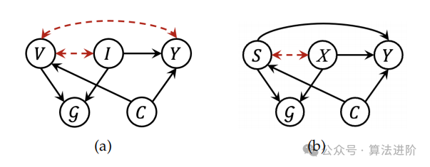
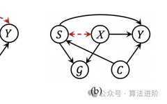
Figure 1 illustrates two causal graphs describing the graph generation process in graph or node-level tasks. G represents the target graph or the neighboring subgraph around the target node, Y represents the labels or model predictions, and C represents (hidden) confounding factors. The black solid arrows indicate causal relationships, while the red dashed arrows indicate spurious correlations. Figure (a) helps reveal the reasons for the poor OOD generalization and interpretability of GNNs, where V and I represent the variants and invariant latent factors of the generated subgraph, respectively. Figure (b) helps reveal the origins of unfairness in graphs, where S and X represent sensitive and insensitive subgraph attributes, respectively.
4 Causal-Inspired Graph Neural Networks (CIGNNs)
Causal-inspired Graph Neural Networks are a causal relationship-based learning approach aimed at improving the performance and generalization ability of neural networks by analyzing causal relationships. These networks typically employ deep learning techniques to optimize network structures and parameters by learning causal relationships, thereby better adapting to complex data and tasks.
Causal-inspired neural networks have applications in various fields, such as natural language processing, computer vision, and reinforcement learning. They can be used to solve problems that traditional methods struggle to handle, such as causal inference and causal prediction. By analyzing causal relationships, causal-inspired neural networks can better understand data and tasks, thereby better adapting to and solving various problems.
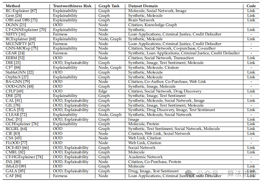
Understanding the causal relationships underlying the data is crucial for developing reliable GNNs. This section provides a systematic review of existing CIGNNs and uses a classification system to highlight their different causal learning capabilities. Figure 2 presents a detailed classification of existing CIGNNs based on their enhanced causal learning capabilities, while Table 1 summarizes the key features of the reviewed works.
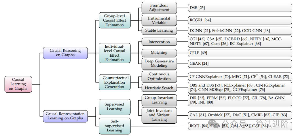
Figure 2 presents a detailed classification of existing CIGNNs based on their enhanced causal learning capabilities.
Table 1 summarizes the reviewed CIGNNs.
4.1 Causal Task-Oriented Classification
Existing CIGNNs enhance reliability by equipping GNNs with causal learning capabilities, mainly divided into causal inference and causal representation learning. Causal inference aims to estimate causal effects between different graph components, including labels and model predictions, using this causal knowledge to enhance the reliability of Graph Neural Networks. Causal representation learning explores the ability of Graph Neural Networks to learn causal representations directly from raw graph data, seamlessly integrating the causal learning process into the standard problem-solving workflow of Graph Neural Networks.
4.2 Enhancing Causal Inference Capabilities of Graphs
Enhancing the causal inference capabilities of Graph Neural Networks aims to improve their reliability by quantifying the causal relationships between graph components and the outcomes of interest (e.g., labels and model predictions). Here, we focus on three noteworthy causal inference problems on graph data, including population-level causal effect estimation, individual-level causal effect estimation, and counterfactual explanation generation.
4.2.1 Population-Level Causal Effect Estimation
In Graph Neural Networks, population-level causal effect estimation is an important causal inference method aimed at quantifying the relationships between different graph components and the target variable. Population-level causal effect estimation can help improve the OOD generalization and interpretability of Graph Neural Networks. In terms of OOD generalization, by learning the causal effects of different graph features on the target labels, Graph Neural Networks can identify and rely on those graph features with strong causal effects to achieve generalization performance. In terms of interpretability, accurate estimation of the causal effects of model predictions aids in more reliable attribution.
The main challenge faced by population-level causal effect estimation is how to control the confounding factors between treatment and outcome variables. Due to the complexity of graph data, traditional backdoor adjustment methods may be impractical. To address this issue, researchers have proposed three methods to circumvent the above challenges. Among them, the first two methods adopt classic causal identification strategies, while the third method employs generative models.
4.2.1 Individual-Level Causal Effect Estimation
Individual-level causal effect estimation is a causal inference method aimed at inferring the potential outcomes for each node or graph instance. This method can help eliminate spurious interpretability and primarily focuses on inferring the counterfactual results for each node. Individual-level causal effect estimation can be achieved through three methods: intervention, matching, and generative models.
Intervention can repeatedly intervene on graph data without ethical or cost issues to eliminate spurious interpretability. Matching is a similarity-based method that eliminates spurious interpretability by matching nodes with similar features. Generative models are deep learning-based methods that infer the potential outcomes for each node by generating counterfactual results. All three methods can infer the counterfactual results for each node, thereby eliminating spurious interpretability. The first two methods are classic causal techniques, while the last method is based on deep learning.
4.2.3 Graph Counterfactual Explanation Generation (GCE)
Graph Counterfactual Explanation Generation is a method for generating counterfactual results aimed at inferring the potential outcomes for each node. This method can eliminate spurious interpretability as it can infer the counterfactual results for each node. GCE answers the question, “What is the minimum perturbation of the input graph sample required to change the model prediction?” revealing necessary features and providing valuable suggestions to users. GCE complements factual explanations, measuring the contributions of graph features from both model-driven and user-driven perspectives. GCE can enhance the post-hoc interpretability of GNNs and provide valuable suggestions in many real-world scenarios.
4.3 Enhancing Causal Representation Learning (CRL) of Graphs
Integrating CRL into Graph Neural Networks holds great potential. The ability of Graph Neural Networks to capture nonlinear relationships is beneficial for latent variable representation learning, while CRL can abstract high-level causal variables with invariant causal effects on the outcomes of interest from fine-grained graph components. These causal representations can be used for generalized predictions or generating faithful explanations for Graph Neural Networks. Furthermore, Graph Neural Networks combined with CRL naturally exhibit better inherent interpretability.
In this section, we first introduce the fundamentals of invariance learning, which plays a key role in the current literature on graph CRL. We then detail how existing works empower Graph Neural Networks with the ability to learn causal representations through supervised or self-supervised learning.
4.3.1 Fundamentals of Invariance Learning
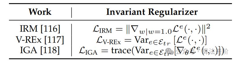
Invariance learning is an important learning method aimed at learning causal relationships that are independent of the data environment, with the fundamental assumption being the invariance of causal mechanisms. The goal is to improve the reliability and interpretability of models. We propose an important assumption that causal mechanisms are constant, meaning that the causal relationships between the target variable Y and its direct causal parents are constant. However, Invariant Causal Prediction (ICP) is limited in the causal relationships between the original features and target labels. Invariant Risk Minimization (IRM) extends ICP to handle potential causal mechanisms and inspires a series of invariant learning methods with the help of representation learning. The invariance assumption of IRM is that there exists a data representation Φ(X) such that ∀e,e’∈Etr,E[Y|Φ(Xe)]=E[Y|Φ(Xe’)]. To find such a Φ(X), IRM is based on the fact that landmarks of Φ(X) correspond to the optimal invariant predictor w(·) on Etr, based on this fact, IRM is based on the following optimization problem: minimizing the constrained problem of Φ(X) and w in the empirical loss L e(·,·) in the environment e∈Etr. We adopt several representative works that have been utilized in graph CRL, as shown in Table 2.
Table 2 presents three commonly used invariant regularization terms.
4.3.2 Supervised Causal Representation Learning
In supervised causal representation learning, we utilize the supervisory signals from downstream tasks to guide the learning process of GNNs and shape the representation space. IRM is a paradigm of learning from multiple data environments, and with its rising trend, many researchers have designed advanced models to obtain supervised signals from downstream tasks, primarily focusing on learning invariant graph representations. In this context, we highlight two representative works.
Group Invariant Learning aims to extend invariant learning to more practical scenarios where explicit labels are unavailable across different environments. The key idea is to infer different training environments using disentangled representations from input graphs (s), thereby satisfying the requirements of invariant learning. DIR[23] implements the idea of group invariant learning to improve graph-level tasks. EERM[52] was the first attempt at group invariant learning in node-level tasks.
FLOOD[77] posits that GNN-based invariant encoders should generalize well to distribution shifts and should adapt to testing data rather than remaining invariant during training and testing phases. GIL [78] effectively adopts Heterogeneous Risk Minimization (HRM) [121], a novel group invariant learning method that theoretically describes the role of environments in learning invariant causal representations in graph-level tasks. BA-GNN [79] adopts a similar idea to enhance node-level tasks. INL[80] further replaces K-means with a contrastive modular graph clustering strategy to enhance the environmental inference module.
Joint Invariance and Variability Learning is a method that separates invariant variables I and variable variables by more direct supervisory objectives. CAL designs an attention-based disentanglement module that generates representations hI and hV for I and V, respectively, which are then passed to invariant predictors and variability predictors, guiding hI to capture invariant causal information through supervised classification loss and guiding hV to capture non-causal variability patterns by pushing wV(hV) to approximate uniform distribution. CMRL adopts the same idea to enhance GNNs’ ability to identify substructures that influence relationships between molecules. Orphicx adopts this idea to learn causal representations I with maximum causal information flow to model predictions ˆY. CIE replaces the variability representation supervisory loss in CAL with promoting independence between disentangled hI and hV from input graphs. DisC performs a similar disentanglement strategy to generate hI and hV and employs invariant predictors and variant predictors to facilitate the learning of hI and hV.
4.3.3 Self-Supervised Causal Representation Learning
Self-supervised learning guides representation learning through unsupervised supervisory signals to retain causal relationships. GCL methods utilize similarity measures based on mutual information, such as InfoNCE and SimCLR, to promote the learning of discriminative representations in Graph Neural Networks. RGCL designs a graph enhancement method considering invariance to stimulate GCL’s potential for learning invariant causal representations on graphs. CIGA theoretically analyzes the importance of comparing invariant representations across different data environments to eliminate the variance information in estimating invariant representations under graph distribution shifts with certain SCMs. GALA assumes that for any variant graph component V, there exist two data environments e1, e2∈Etr such that P e1(Y|V)=P e2(Y|V), but P e1(Y|I)=P e2(Y|I). It then employs a bias model training based on the correctness of model predictions to find these data environments. IMoLD counterfactually perturbs the disentangled variant factors V from the input graphs to other graphs to create a view set sharing the same invariant factors I, maximizing the similarity among them to facilitate the learning of I and V. CAF enhances the GNN’s GCF by utilizing sensitive attribute-aware counterfactual augmentation for each node.
5 Datasets
To ensure the validity of the validation, it is essential to understand the details of the datasets and select appropriate datasets that exhibit diversity. The graph generation processes in different applications may lead to different types of distribution shifts, unfairness, or model interpretability issues, making the diversity of datasets crucial. Next, we will introduce existing real-world and synthetic datasets that have been used for evaluating reliability across three aspects.
5.1 Datasets for Evaluating OOD Generalizability
5.1.1 Benchmark Datasets
To evaluate the performance of GNNs at the node and graph levels, researchers have utilized various real-world and synthetic graph datasets. These datasets come from diverse sources and cover a wide range of features and structures. Li et al. provide a summary of the datasets and key statistics. Gui and Li et al. created an advanced graph OOD benchmark, GOOD, to compare different graph OOD methods. It includes six graph-level and five node-level datasets, generated through unbiased, covariate shift, and concept shift divisions. Ji and Zhang et al. organized an AI-assisted drug discovery benchmark aligned with biochemical knowledge for evaluating graph OOD generalization methods. Wang and Chen et al. developed an OOD dynamics attribute prediction benchmark that exhibits distribution shifts across multiple dimensions.
5.1.2 Specialized Data Synthesis
To evaluate the generalization ability of GNNs, it is necessary to synthesize distribution-shifted data of varying severity. Existing benchmark graph OOD datasets exhibit diversity but contain spurious correlations. Multiple levels of distribution shifts can be created by adjusting data selection biases and generating spurious features influenced by counterfactual labels. Adjusting data selection biases includes sampling invariant subgraphs from uniform distributions and introducing data selection biases to adjust P(V|I), while generating spurious features involves labeling nodes for a given graph and generating spurious node features for environment i. These methods help evaluate the performance of GNNs on OOD.
5.2 Datasets for Evaluating Graph Fairness
5.2.1 Benchmark Datasets
Benchmark datasets for graph fairness research are generated to include examples of potential biases and unfairness, such as underrepresented groups or imbalanced classes. The datasets need to consider factors beyond traditional graph learning benchmarks. Dong et al. summarize benchmark graph fairness datasets and classify them into social networks, recommendation-based graph networks, academic networks, and other types of networks.
5.2.2 Specialized Data Synthesis
Assessing the fairness of Graph Neural Networks on real-world datasets faces two limitations: the need to define sensitive attributes and obtain true counterfactual graphs required for evaluation. Therefore, controllable synthetic graph datasets are needed. Ma et al. synthesized data based on causal models for evaluating GCF, sampling sensitive attributes from Bernoulli distributions, with node features and graph structures generated from latent factors. Guo et al. also utilized this data synthesis idea to generate node features with constant parts only influenced by Yi and variant parts only influenced by Si. These methods help evaluate the fairness of Graph Neural Networks.
5.3 Datasets for Evaluating Graph Explanations
To evaluate the performance of factual and counterfactual graph explainers, it is necessary to collect datasets of various sizes, types, structures, and application scenarios. Graph datasets should meet two criteria: human-understandable, easy to visualize, and capable of identifying expert knowledge. This aids in the quantitative evaluation of explainers. In relevant studies, a comprehensive analysis of commonly used synthetic graphs, sentiment graphs, and molecular graphs for evaluating the quality of factual graph explanations has been conducted, which are also used for evaluating counterfactual explanations.
6 Evaluation Metrics
The choice of evaluation metrics is crucial for a comprehensive and accurate assessment of the proposed models. Using a single metric may lead to potential biases or errors. Researchers typically prioritize metrics related to accuracy, such as accuracy, ROC-AUC, F1 score, and precision. However, these metrics may not reveal the reliability of the model. Therefore, several TGNN metrics have been proposed to evaluate the model. These metrics can provide a more comprehensive assessment and help ensure the practicality of the model in graph-related applications.
6.1 Metrics for Evaluating OOD Generalization Ability of Graphs
To evaluate the generalizability of OOD, accuracy-related metrics can be compared across different distribution-shifted testing environments. In high-risk application fields, such as criminal justice and finance, there is a tendency to assess the overall stability or robustness of models across various OOD scenarios. To this end, several metrics are listed, including average accuracy (which measures the average performance across all testing environments), standard deviation accuracy (which measures performance variation across all testing environments), and worst-case accuracy (which reflects the worst results that methods may produce). The first two metrics provide a broader perspective on OOD stability, while the last metric is more applicable in applications where extreme performance is unacceptable.
6.2 Metrics for Evaluating Graph Fairness
This section proposes various metrics to assess the fairness of GNNs, including statistical parity, equal opportunity, etc. These metrics primarily focus on the differences in model predictions among groups with different sensitive attributes. Since counterfactual fairness is considered a more comprehensive concept, it is necessary to evaluate the performance of GNNs optimized for GCF on these correlation-based fairness metrics. Additionally, the GCF concept also induces causal relationship-based metrics, such as unfairness scores and GCF metrics. The unfairness score is defined as the percentage of nodes whose predicted labels change when altering the sensitive attributes of nodes. The GCF metric measures the differences between the intervention distributions of model predictions rather than the differences between node representations, while considering the impact of sensitive attributes of nodes and their neighbors on model fairness.
6.3 Metrics for Evaluating Graph Interpretability
To explain the behavior of models, graph explanations are generated to elucidate model behavior, and several evaluation metrics are proposed from the model’s perspective. These metrics include fidelity, sparsity, stability, contrast, sufficiency probability, and accuracy. These metrics are applicable to both factual and counterfactual graph explanation methods. To generate GCEs, maintaining similarity with the original input graph is crucial, so appropriate metrics must be adopted from this perspective to evaluate GCEs. Similarity/distance measures such as graph edit distance and Tanimoto similarity have been employed. Additionally, Lucic et al. proposed customized MEG similarity, Liu et al. defined counterfactual relevance, and Tan et al. proposed necessity probability. Furthermore, the above metrics can be extended to scenarios where multiple GCEs are generated for each input graph. Additionally, metrics have been proposed to evaluate GCEs from other perspectives beyond their basic definitions. Ma et al. designed causal ratios, and Huang and Kosan et al. proposed coverage, cost, and interpretability.
7 Future Directions
We will explore several future research directions aimed at investigating how to integrate causal learning into GNNs to enhance their reliability.
(1) Expanding CIGNNs to Accommodate Large-Scale Graphs.Due to the high computational cost of GNNs in messaging schemes, scaling to large-scale graphs is challenging. Although many scalable GNNs have been proposed, there is still a significant gap in research regarding CIGNNs. On one hand, the techniques employed in CIGNNs may not scale to large-scale graphs. For instance, graph perturbations used to create multiple counterfactual graphs [24],[52] lead to increased computational costs as the graph size increases. On the other hand, techniques designed for scalable GNNs may not seamlessly integrate into CIGNNs. For example, sampling strategies in GNN messaging inevitably disturb the invariant and variable components in the node neighborhood, raising concerns for causal learning methods. Further exploration of the scalability of CIGNNs is needed.
(2) Causally-Inspired Graph Foundation Models. The success of large language models (LLMs) has driven the development of graph foundation models pre-trained on various graph data, and integrating causal relationships into the development of large reliable graph models is a promising direction. However, the effectiveness of existing causally-inspired methods is questioned on large models, as these methods are mainly evaluated on smaller GNNs. For instance, graph invariant learning methods may overfit on large models. Given the potential of large graph models in changing the paradigm of graph learning, existing work must be critically assessed, and new causal-based methods should be explored to enhance the reliability of large graph models.
(3) Discovering Causal Relationships on Graphs. The causal reasoning and causal representation learning capabilities of Graph Neural Networks can enhance their reliability, but domain knowledge is required to abstract meaningful causal reasoning tasks. In the absence of domain knowledge, the effectiveness of causal representation learning relies on additional assumptions about the underlying graph generation mechanisms. Causal discovery can identify causal relationships between variables in a data-driven manner, supplementing the missing domain knowledge and examining the assumptions of data causality. The discovered causal knowledge can be infused into Graph Neural Network models to facilitate learning semantically meaningful and identifiable graph representations. Therefore, equipping Graph Neural Networks with causal discovery capabilities holds great potential for developing Graph Neural Network models that perform well in various application scenarios.
(4) Beyond Graph Counterfactual Fairness. The GCF concept measures the fairness of Graph Neural Networks through the total causal effect of sensitive attributes on output node representations. However, the GCF concept is no longer applicable in the presence of unfairness, as sensitive attributes may influence outcomes along certain causal paths. To address this issue, intervention fairness concepts and counterfactual fairness concepts specific to certain paths have been proposed to capture the most prominent causal mechanisms in practical applications. Nevertheless, these concepts have not yet been utilized to improve graph fairness, so it is necessary to develop causal relationship-based graph fairness concepts that go beyond GCF.
(5) Causally-Based Privacy Protection. Privacy protection imposes additional constraints on GNNs, intersecting with the causality of AI. Vo et al. studied counterfactual explanations for privacy protection, but there is a lack of research on the compatibility of CIGNN systems with privacy protection from the perspective of privacy protection in the literature. Therefore, it is worthwhile to explore the compatibility of existing CIGNNs with privacy protection technologies to establish trustworthy GNN systems suitable for privacy-critical scenarios.Edited by: Huang Jiyan