A Comprehensive Guide to Understanding RNN Family

BERT is great, but don’t forget our old friend RNN!

Introduction

CNN (Convolutional Neural Network) and RNN (Recurrent Neural Network) are two mainstream structures in the field of Deep Learning applications today. In the previous article, we introduced CNN, and in this article, we will discuss RNN. RNN and CNN share a similar history as concepts proposed in the last century. However, due to the lack of computational power and data at that time, they were both shelved until they began to shine in recent years, making them products ahead of their time. The difference is that CNN started to gain popularity in 2012, while RNN did not become popular until after 2015. This article will introduce relevant concepts of RNN and specifically discuss common RNN architectures.

Original RNN

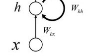
One of the characteristics of CNN architecture is that the network’s state only depends on the input, while RNN’s state depends not only on the input but also on the state of the network at the previous moment. Therefore, it is often used to handle sequence-related problems. The basic structure of RNN is as follows: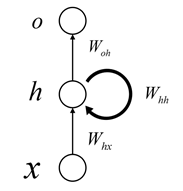

As can be seen, the difference between it and Feedforward Neural Network structures like CNN and DNN lies in that: Feedforward NN is structured as a DAG (Directed Acyclic Graph), while Recurrent NN has at least one loop. Assuming that state transitions occur in the time dimension, the above diagram can be expanded as follows: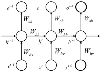

Thus, we can write its specific expression:

where represents the input at time t, represents the output at time t, and represents the state of the Hidden Layer at time t.

RNN and BPTT

The training of RNN is essentially the same as that of CNN and DNN, still using backpropagation. However, its backpropagation method has a more advanced name called BPTT (Back Propagation Through Time).

First, let’s review some concepts related to DNN. The structure of DNN is shown in the following diagram: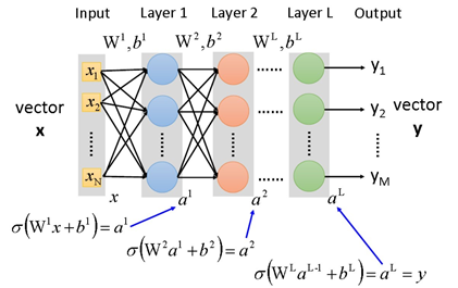

The most important formula in DNN’s backpropagation is as follows (not elaborated here):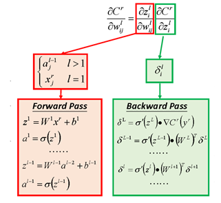

With the above conclusions from DNN, we can unfold RNN along the time dimension (UNFOLD), as shown in the following diagram: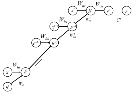

It can be observed that the unfolded RNN is actually logically the same as DNN, but the connections between adjacent layers in DNN become connections between adjacent time steps in RNN, so the formulas are also quite similar. However, one point to note is that for a certain parameter, if we only consider the loss at time t, its gradient is the accumulated gradient throughout the entire backpropagation process after unfolding, as represented by the following formula. Where represents the state at time t.

Similarly, if we consider the total error, we have:

The above formula can be described more intuitively with the following slide from Professor Li Hongyi’s PPT: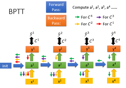

Now, if we only consider , we can observe the structure of the unfolded RNN network. Referring to the DNN’s backpropagation formula, we can directly write the BPTT formula for the original RNN as follows:

RNN and Gradient Vanish / Gradient Explode

The BPTT formula of RNN is very similar to that of DNN, so it undoubtedly faces the problems of Gradient Vanish and Gradient Explode. There are mainly two reasons for this:

1. Activation Function

In the above formula, if the activation function is a sigmoid or tanh function, according to the recurrence relation, when the time span is large (corresponding to a very deep DNN), it will become very small, resulting in Gradient Vanish during backpropagation. The solution is similar, using a different Activation Function, such as Relu, etc.

2. Parameters

Unlike DNN where each layer’s parameters are relatively independent, in RNN, the parameters at each time step actually refer to the same parameter, leading to the accumulation of multiplications in .

When it is a diagonal matrix, we have two conclusions:

• If some diagonal elements are less than 1, their powers will approach 0, leading to Gradient Vanish.
• If some diagonal elements are greater than 1, their powers will approach infinity, leading to Gradient Explode.

Of course, it is not necessarily a diagonal matrix; if it is a non-diagonal matrix, we will illustrate it through experiments. First, we randomly initialize the values of . Then we observe how the distribution of values changes as we multiply them multiple times as shown in the following diagram. It can be seen that after multiple multiplications, the distribution of values shows a clear trend: either approaching 0 or approaching a very large absolute value. These two cases can likely cause Gradient Vanish and Gradient Explode respectively: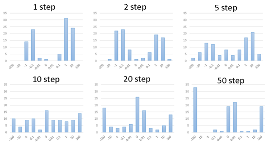

The methods to solve Gradient Vanish and Gradient Explode are as follows:

• For Gradient Vanish, traditional methods are effective, such as changing the Activation Function; however, a better architecture can significantly alleviate this issue, such as LSTM and GRU introduced below.
• For Gradient Explode, a common approach is to limit the gradient within a certain range, known as Gradient Clipping. This can be done through a threshold or dynamic scaling.

BRNN

BRNN (Bi-directional RNN) was proposed by Schuster in “Bidirectional recurrent neural networks, 1997” and is an extension of unidirectional RNN. Ordinary RNN only focuses on the previous context, while BRNN simultaneously focuses on both the previous and following contexts, allowing it to utilize more information for predictions.

Structurally, BRNN consists of two RNNs that operate in opposite directions, both connected to the same output layer. This achieves the goal of simultaneously focusing on the context. Its specific structure diagram is as follows: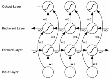

BRNN is essentially the same as ordinary RNN, with only slight differences in training steps and other details, which will not be elaborated here. Interested readers can refer to the original text.

LSTM

To solve the issue of Gradient Vanish, Hochreiter & Schmidhuber proposed LSTM (Long Short-Term Memory) in their paper “Long short-term memory, 1997”. The original LSTM only had Input Gate and Output Gate. The LSTM we commonly refer to now also includes the Forget Gate, which is an improved version proposed by Gers in “Learning to Forget: Continual Prediction with LSTM, 2000”. Later, in “LSTM Recurrent Networks Learn Simple Context Free and Context Sensitive Languages, 2001”, Gers introduced the concept of Peephole Connection. Additionally, modern deep learning frameworks like TensorFlow and PyTorch have some subtle differences in their implementations of LSTM. Although they all essentially represent LSTM, there are structural differences to note during usage.

The LSTM introduced below is the “Traditional LSTM with Forget Gates” version.

Traditional LSTM with Forget Gates

LSTM is essentially replacing a neuron in the Hidden Layer of RNN with a more complex structure called a Memory Block. The structure of a single Memory Block is as follows (the dashed lines in the figure represent Peephole Connections, which can be ignored):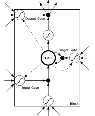

Here is a brief introduction to the structure:

• Input Gate, Output Gate, Forget Gate: These three Gates are essentially weights, and to visualize, they are similar to switches in a circuit that control current flow. When the value is 1, it indicates that the switch is closed, and the flow passes without loss; when the value is 0, the switch is open, completely blocking the flow; when the value is between (0,1), it indicates the degree of flow passing. The values are actually implemented using the Sigmoid function.
• Cell: The Cell represents the current state of the Memory Block, corresponding to the neurons in the Hidden Layer of the original RNN.
• Activation Function: The figure shows multiple Activation Functions (small circles with sigmoid curve patterns). There is a general standard for selecting these Activation Functions. Generally, for Input Gate, Output Gate, and Forget Gate, the Activation Function used is the sigmoid function; for Input and Cell, the Activation Function used is the tanh function.

The specific formulas are as follows:

where represent Input Gate, Output Gate, Forget Gate; represent Input; represent Output; represent the state of the Cell at time t.

LSTM and Gradient Vanish

As mentioned above, LSTM was proposed to solve the Gradient Vanish problem of RNN. The fundamental reason for Gradient Vanish in RNN has been clearly introduced above, mainly due to the high powers of matrices. Below, we briefly explain why LSTM can effectively avoid Gradient Vanish.

For LSTM, the following formulas apply:

Imitating RNN, we compute LSTM, yielding:

The other terms in the formulas are not important, represented here by ellipses. It can be seen that even if the other terms are very small, the gradient can still be well propagated to the previous moment; even when the layers are deep, Gradient Vanish will not occur; when the signal from the previous moment does not affect the current moment, this term will also be 0; here controls the decay of the gradient propagation to the previous moment, consistent with the function of the Forget Gate.

LSTM and BPTT

When LSTM was first proposed, its training method was “Truncated BPTT”. This means that only the state of the Cell would backpropagate multiple times, while other parts’ gradients would be truncated and not passed back to the previous moment’s Memory Block. Of course, this method is no longer used, so it’s mentioned here only in passing.

In “Framewise phoneme classification with bidirectional LSTM and other neural network architectures, 2005”, the authors proposed Full Gradient BPTT to train LSTM, which is the standard BPTT. This is also the method used by modern open-source frameworks with automatic differentiation capabilities. Regarding LSTM’s Full Gradient BPTT, I have not derived the specific formulas, but interested readers can refer to the idea of UNFOLD in RNN to try it out; I will not elaborate further here.

GRU

GRU (Gated Recurrent Unit) was proposed by K. Cho in “Learning Phrase Representations using RNN Encoder–Decoder for Statistical Machine Translation, 2014”. It is a simplified version of LSTM, but in most tasks, its performance is comparable to LSTM, making it one of the commonly used RNN algorithms.

The specific structure of GRU and its corresponding formulas are as follows: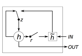

Where they are referred to as Reset Gate and Update Gate. It can be seen that GRU has some similarities to LSTM, while the main differences are:

1. LSTM has three Gates, while GRU has only two.
2. GRU does not have a Cell like LSTM, but directly computes the output.
3. The Update Gate in GRU is similar to the combination of Input Gate and Forget Gate in LSTM; observing the Gates connected to the previous moment in their structures, it can be seen that the Forget Gate in LSTM is actually split into the Update Gate and Reset Gate in GRU.

Many experiments have shown that GRU and LSTM perform similarly, but GRU has fewer parameters, making it relatively easier to train and less prone to overfitting; it can be tried when training data is limited.

Conclusion

Besides the architectures mentioned in this article, RNN has other variations. However, overall, the evolution of RNN architectures is currently lagging behind CNN, with LSTM and GRU being the main commonly used ones. Similarly, since RNN has less to discuss than CNN, this article is dedicated to introducing RNN, and the content has been compressed. However, this does not mean RNN is simple; on the contrary, both theoretically and practically, the difficulty of using RNN is significantly higher than that of CNN.

In the next article (barring any surprises), we will start discussing unsupervised learning related to Deep Learning.