LSTM is a type of time-recursive neural network suitable for processing and predicting important events with relatively long intervals and delays in time series. It has achieved excellent results in a series of applications such as natural language processing and language recognition.

“Long Short Term Memory Networks with Python” is a book by Australian machine learning expert Jason Brownlee, which provides a detailed introduction to the principles and use of the LSTM model.

The book is divided into fourteen chapters, as follows:

Chapter 1: What are LSTMs?

Chapter 2: How to train LSTMs?

Chapter 3: How to prepare data for LSTMs?

Chapter 4: How to develop LSTMs in Keras?

Chapter 5: Sequence prediction modeling

Chapter 6: How to develop a Vanilla LSTM model?

Chapter 7: How to develop Stacked LSTMs?

Chapter 8: Developing CNN LSTM models

Chapter 9: Developing Encoder-Decoder LSTMs

Chapter 10: Developing Bidirectional LSTMs

Chapter 11: Developing Generative LSTMs

Chapter 12: Diagnosing and debugging LSTMs

Chapter 13: How to make predictions with LSTMs?

Chapter 14: Updating LSTM models

The author of this article has organized and translated this book for everyone. We will continue to release a series of articles to introduce the detailed content inside, and learn together with everyone, support for questions! Support for questions! Support for questions!Important things are said three times!

If you have any related questions, you can leave us a message at the bottom of the article! We will definitely reply to you!

This article has about 12,000 words, and it takes 12 minutes to read. It is recommended to bookmark and study.

There are benefits at the end of the article

1.0 Introduction

1.0.1 Course Objectives

The purpose of this course is to give you a higher-level understanding of LSTMs, so that you can explain what they are and how they work.

By the end of this lesson, you will know:

• What sequence prediction is, and how it differs from general predictive modeling problems;

• The limitations of Multilayer Perceptrons (MLPs) for sequence prediction, the guarantees of Recurrent Neural Networks (RNNs) for sequence prediction, and how LSTMs convey those guarantees;

• Some impressive applications of LSTMs that challenge sequence prediction problems, as well as warnings about some limitations of LSTMs.

1.0.2 Course Overview

This course is divided into 6 sections, which are:

1. Sequence prediction problems;

2. Limitations of Multilayer Perceptrons;

3. Guarantees of Recurrent Neural Networks;

4. LSTM Networks;

5. Applications of LSTM Networks;

6. Limitations of LSTM Networks.

Let’s get started!

1.1 Sequence Prediction Problems

Sequence prediction differs from other types of supervised learning problems. Sequence emphasizes the order of observations, and this order must be preserved when training the model and making predictions. Generally, the design of predictive problems for sequential data is referred to as sequence prediction problems, although there are many issues with this terminology based on the differences in input and output order. In this section, we will look at four types of sequence prediction problems:

1. Sequence Prediction;

2. Sequence Classification;

3. Sequence Generation;

4. Sequence-to-Sequence Prediction.

But first, let’s clarify the difference between a set and a sequence.

1.1.1 Sequence

In machine learning applications, we often use sets, such as training sets and test sets. Each sample in a set can be considered an observation from within its range. The order of observations in a set is not important. A sequence, on the other hand, emphasizes the detailed order of observations. Here, the order is very important! When using sequential data as input and output for models, it is essential to be particularly careful in defining the predictive problem!

1.1.2 Sequence Prediction

Sequence prediction involves predicting the next value of a given input sequence. For example:

Input sequence: 1,2,3,4,5
Output sequence: 6

List 1.1: Example of a sequence prediction problem

graph LR
    A["[1,2,3,4,5]"]-->B["Sequence Prediction Model"]
    B["Sequence Prediction Model"]-->C["[6]"]

Figure 1.1 Description of a sequence prediction problem

Sequence prediction problems are often referred to as sequence learning. Technically, we can consider all the problems below as types of sequence prediction problems. This may confuse beginners.

Learning from continuous data remains a fundamental task and challenge in pattern recognition and machine learning. Applications that involve data sequences may require predictions of new events, generation of new sequences, or decisions such as classification of sequences or subsequences.

— On Prediction Using Variable Order Markov Models, 2004.

In general, in this book, we will use “sequence prediction” to refer to this category of predictive problems that involve sequential data. However, in this section, we will distinguish between sequence prediction and other forms of predictions involving sequential data, defining it as predicting the next time step.

Sequence prediction attempts to predict the elements of a sequence based on preceding elements.

— Sequence Learning: From Recognition and Prediction to Sequential Decision Making, 2001.

Some examples of sequence prediction problems include:

• Weather Prediction. Given a sequence of time-based weather observations, predict tomorrow’s weather.

• Stock Prediction. Given a sequence of time-based price fluctuations of a security, predict the price fluctuation of the security tomorrow.

• Product Recommendation. Given a customer’s past shopping history, predict the customer’s next shopping behavior.

1.1.3 Sequence Classification

Sequence classification involves predicting the classification label of a given input sequence. For example:

Input sequence: 1,2,3,4,5
Output sequence: "good"

List 1.2: Example of a sequence classification problem

graph LR
    A["[1,2,3,4,5]"]-->B["Sequence Classification Model"]
    B["Sequence Classification Model"]-->C["good"]

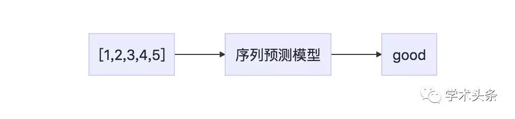
Figure 1.2 Description of a sequence classification problem

The goal of sequence classification problems is to build a classification model using a labeled dataset […] so that the model can predict the classification label of an unseen sequence.

— Discrete Sequence Classification, Data Classification: Algorithms and Applications, 2015.

The input sequence can consist of actual values or discrete values. In the latter case, these problems can be referred to as discrete sequence classification problems. Some examples of sequence classification problems include:

• DNA Sequence Classification. Given DNA sequence values A, C, G, and T, predict whether the sequence is a coding region or a non-coding region.

• Anomaly Detection. Given a sequence of observations, predict whether the sequence is anomalous.

• Sentiment Analysis. Given a sequence of text, such as a review or a tweet, predict whether the sentiment of the text is positive or negative.

1.1.4 Sequence Generation

Sequence generation involves producing a new output sequence that shares characteristics with the sequences in the corpus. For example:

Input sequence: [1,3,5],[7,9,11]
Output sequence: [3,5,7]

List 1.3: Example of a sequence generation problem

graph LR
    A["[1,3,5],[7,9,11]"]-->B["Sequence Generation Model"]
    B["Sequence Generation Model"]-->C["[3,5,7]"]

Figure 1.3 Description of a sequence generation problem

Recurrent Neural Networks (RNNs) can predict sequence generation by processing real data sequences step by step, predicting what will happen next. [Recurrent Neural Networks] can predict sequence generation by processing real data sequences step by step, predicting what will happen next. Assuming predictions are probabilistic, new sequences can be generated from the training network by iteratively sampling from the output distribution of the network and feeding the samples back into the input in the next step. In other words, let the network treat their inventions as realities, just like a person dreams. Relatively new, the seq2seq method has achieved state-of-the-art machine translation in [results].

— Generating Sequences With Recurrent Neural Networks, 2013.

Some examples of sequence generation problems include:

• Text Generation: Given a corpus of text, such as Shakespeare’s literary work, generate new sentences or paragraphs of text that can be extracted from the corpus.

• Handwriting Prediction: Given a handwriting corpus, generate new phrases of handwriting that possess attributes found in the corpus.

• Music Generation: Given a corpus of musical instances, generate new musical segments that share attributes with the corpus. Sequence models can refer to sequence generation based on single observations as input. An example is the automatic text description of images.

• Image Caption Generation: Given an image as input, generate a sequence of words that describes the image.

For example:

Input sequence: [image pixels]
Output sequence: ["A person riding a bicycle"]

List 1.4: Example of a sequence generation problem

graph LR
    A["Image pixels"]-->B["Sequence Generation Model"]
    B["Sequence Generation Model"]-->C["A person riding a bicycle"]

Figure 1.4 Description of a sequence generation problem

Automatically describing the content of an image using appropriate sentences is a very challenging task, but it can have a significant impact […]. Indeed, a description must not only capture the objects included in the image but also represent how these objects are related, along with their attributes and the activities they are involved in.

— Show and Tell: A Neural Image Caption Generator, 2015.

1.1.5 Sequence-to-Sequence Prediction

Sequence-to-sequence prediction involves giving an input sequence and predicting an output sequence, for example:

Input sequence: 1,2,3,4,5
Output sequence: 6,7,8,9,10

List 1.5: Example of a sequence-to-sequence problem

graph LR
    A["Image pixels"]-->B["Sequence Generation Model"]
    B["Sequence Generation Model"]-->C["A person riding a bicycle"]

Figure 1.5 Description of a sequence-to-sequence problem

Although deep neural networks are flexible and powerful, they can only be applied to problems where the input and target can be clearly encoded as fixed-dimensional vectors. This is a clear limitation because many important problems are best represented by using sequences of unknown lengths, without a known prior. For example, cause identification and machine translation are continuous problems. Similarly, question answering can be seen as mapping a sequence of words representing a question to a sequence of words representing an answer.

— Sequence to Sequence Learning with Neural Networks, 2014.

Sequence-to-sequence prediction is a subtle and challenging extension of sequence prediction. Instead of predicting a single next value in a sequence, a new sequence is predicted that may or may not have the same length or timing as the input sequence. This type of problem has seen much research recently in the area of automatic text translation (e.g., translating English to grammar) and can be abbreviated as seq2seq. Seq2seq learning, at its core, uses recurrent neural networks to map variable-length input sequences to variable-length output sequences.

— Multi-task Sequence to Sequence Learning, 2016.

If both the input and output sequences are time series, then the problem can be referred to as multi-step time series prediction. Some examples of sequence-to-sequence problems include:

• Multi-step Time Series Prediction. Given a series of time observations, predict a series of future time step observations.

• Text Summarization. Given a text document, predict a shorter text sequence that describes the highlights of the source document.

• Program Execution. Given a text description of a program or mathematical equation, predict the character sequence of the correct output.

1.2 Limitations of Perceptrons

Traditional neural networks are called perceptrons (Multilayer Perceptrons, or MLPs), which can be used for predictive problems in sequence models. MLPs approximate the mapping function from input variables to output variables. For a variety of reasons, their overall capability is useful for sequence prediction problems (especially time series prediction).

• Robust to Noise. Neural networks are very robust to noise in the input data and mapping functions, even supporting learning and prediction in the presence of missing values.

• Non-linearity. Neural networks make no strong assumptions about the mapping function, making it easy to learn linear and non-linear relationships.

Moreover, in the mapping function, MLPs can be configured to support any number of inputs and outputs, but with a certain number of inputs and outputs. This means:

• Multivariate Input. Any number of inputs can be specified, providing direct support for multivariate prediction.

• Multi-step Output. Any number of outputs can be specified, providing direct support for multi-step or even multivariate prediction.

Their capabilities overcome the limitations of traditional linear methods (such as ARIMA for time series prediction). With these capabilities alone, feedforward neural networks are widely used for time series prediction.

The ARIMA model stands for Autoregressive Integrated Moving Average Model. The basic idea of the ARIMA model is to view the data sequence generated by the predicted object over time as a random sequence, approximated by a certain mathematical model. Once this model is identified, it can predict future values based on past and present values of the time series.

A significant contribution of neural networks is their ability to elegantly approximate any non-linear function. This property has high value in time series processing and ensures more powerful applications, especially in the subfield of prediction…

— Neural Networks for Time Series Processing, 1996.

MLPs’ application in sequence prediction requires that input sequences be divided into smaller overlapping subsequences, which are presented to the network to generate a prediction. The time steps of the input sequence become the input features to the network. The subsequences are overlapping to simulate a sliding window along the sequence to generate the desired output. This works well on some problems, but it has five key limitations:

• Stateless. MLPs learn an approximation of a fixed function. Any conditional output in the context of the input sequence must be generalized and fixed to the network’s weights.

• No Awareness of Temporal Structure. Time steps are modeled as input features, meaning the network has no explicit handling or understanding of the temporal structure or order between observations.

• Scale Confusion. For problems requiring modeling multiple parallel input sequences, the number of input features increases as an element of the sliding window size without any explicit separation of time series.

• Fixed Size Input. The size of the sliding window is fixed and must be imposed on all inputs.

• Fixed Size Output. The size of the output is also fixed, and any mismatched output must be forced to be of fixed size.

MLPs indeed provide significant capabilities for sequence prediction, but they are still limited by the overall key limitation that the range of temporal dependencies between observations must be explicitly specified in the model design.

Sequence-to-sequence poses challenges for deep neural networks because they require that the number of input and output dimensions be known and fixed.

— Sequence to Sequence Learning with Neural Networks, 2014.

MLPs are a good starting point for modeling sequence-to-sequence problems, but we now have better options.

1.3 Guarantees of Sequence Models

Long Short-Term Memory, or LSTM networks, are a type of recurrent neural network. Recurrent Neural Networks (RNNs) are a special type of neural network used for sequence problems. Given a standard feedforward MLP network, RNNs can be thought of as adding loops to the architecture. For example, in a given layer, each neuron can gradually (laterally) pass its signal, in addition to forwarding to the next layer. The output of the network can be fed back into the network as the next input vector, and so on.

Recurrent connections add state or memory to the network, allowing it to learn and leverage the ordered nature of observations in the input sequence.

Recurrent neural networks contain loops that feed the previous stage’s network activation back into the network as input to influence the current stage’s predictions. These activations are stored in the internal state of the network, which can, in principle, maintain long-term contextual information. This mechanism allows RNNs to leverage a dynamically changing contextual window over the history of input sequences.

— Long Short-Term Memory Recurrent Neural Network Architectures for Large Scale Acoustic Modeling, 2014.

The sequence’s increase is a new dimension of the function being approximated. The network can learn a time-based mapping function from input to output rather than simply mapping input to output. The internal memory can represent the recent context based on the observations in the input sequence at the time of output, rather than just what has been presented as input to the network. In a sense, this capability unlocks the time series potential of neural networks.

Long Short-Term Memory (LSTM) can solve many tasks that cannot be addressed by feedback networks using fixed-size time windows.

— Applying LSTM to Time Series Predictable through Time-Window Approaches, 2001.

In addition to the general approach of using neural networks for sequence prediction, RNNs can learn and utilize the temporal dependencies of the data. That is, in the simplest case, the network displays one observation at one time in a sequence and can learn how previously observed observations are relevant and how they predict relevance.

Due to the ability to learn long-term correlations in sequences, LSTM networks avoid the need to pre-specify time windows and can accurately model complex multivariate sequences.

— Long Short Term Memory Networks for Anomaly Detection in Time Series, 2015.

The guarantee of recurrent neural networks is that temporal dependencies and contextual information in the input data can be learned.

The input to recurrent neural networks is not fixed but constitutes a sequence that can be used to transform an input sequence into an output sequence while considering contextual information in an understandable manner.

— Learning Long-Term Dependencies with Gradient Descent is Difficult, 1994.

There are many types of RNNs, but it is LSTM that conveys the guarantees of RNNs in sequence prediction. This is why LSTM has so many applications and voices today.

LSTMs have internal states that explicitly recognize the temporal structure in the input, can model multiple parallel input sequences separately, and can produce variable-length output sequences through different lengths of input sequences, observing one time at a time.

Next, let’s take a closer look at LSTM networks.

1.4 LSTM Networks

LSTM networks are different from traditional MLPs. Like MLPs, the network consists of layers of neurons. Input data is propagated through the network for prediction. Unlike RNNs, LSTMs have a unique formulation that prevents issues that hinder other RNNs from scaling and blocking. This, along with impressive results, is what has made this technology popular.

A key problem faced by RNNs has always been how to effectively train them. Experiments have shown that the weight update process leads to weight changes, and weights quickly become so small that they become ineffective (gradient vanishing) or become so large that they lead to very large changes or overflow (gradient explosion), which is a very difficult problem. LSTMs overcome this challenge through design.

Unfortunately, the range of contextual information that standard RNNs can access is very limited. The problem is that given an input on the hidden layer, and thus the output on the network, when it cycles around the recurrent connections of the network, it either exponentially decays or exponentially rises. This drawback… is referred to in the literature as the gradient vanishing problem… Long Short-Term Memory (LSTM) is an RNN architecture designed to solve the gradient vanishing problem.

— A Novel Connectionist System for Unconstrained Handwriting Recognition, 2009.

The computational units of LSTM networks are called memory cells, memory blocks, or simply cells. When describing MLPs, the term “neuron” is deeply rooted as the computational unit, so it is often used to refer to LSTM memory cells. An LSTM cell consists of weights and gates.

The long-short structure is achieved by analyzing the errors in existing RNNs, finding that long-time lags are inaccessible to existing architectures because the backpropagation errors either exponentially rise or decay. The LSTM layer consists of a set of recursively connected blocks called memory blocks. These blocks can be thought of as differentiable versions of storage chips in digital computers. Each contains one or more recursively connected memory cells and a single multiplication unit—input gate, output gate, and forget gate—providing continuous simulation of write, read, and reset operations for the cell. The network can only interact with the cell through gates.

— Framewise Phoneme Classification with Bidirectional LSTM and Other Neural Network Architectures, 2005.

1.4.1 LSTM Weights

A memory cell has input and output weight parameters, as well as an internal state established by exposure to input time steps.

• Input Weights. Used to weight the input at the current time step.

• Output Weights. Used to weight the output from the last step.

• Internal State. Used in the output computation at this time step.

1.4.2 LSTM Gates

The key to the memory cell is the gates. These are also weighted functions that further control the information in the cell. There are three gates:

• Forget Gate. Determines what information needs to be discarded from the cell.

• Input Gate. Determines which values from the input are used to update the memory state.

• Output Gate. Determines what to output based on the input and the cell’s memory.

The forget gate and input gate are used in the internal state update. The input gate is the final constraint on what the cell actually outputs. It is these gates and the consistent data flow referred to as CEC (constant error carousel) that keep each cell stable (neither exploding nor vanishing).

The internal structure of each memory cell guarantees CEC (its constant error carousel). This indicates bridging the fundamental lags for a long time. Two gate units learn to open and close access to errors in each memory cell’s CEC. The multiplicative input gate protects the CEC from disturbances due to irrelevant inputs. Similarly, the multiplicative output gate protects other cells from interference from the current irrelevant memory content.

— Long Short-Term Memory, 1997.

Unlike traditional MLP neurons, it is challenging to draw a clean LSTM memory cell. There are wires, weights, and gates everywhere. Check out some resources at the end of this chapter if you think that image-based or equation-based descriptions of LSTM internals would help further research. We can summarize three key terms of LSTM as follows:

• Overcoming the technical issues of training RNNs, namely the gradient vanishing and gradient explosion problems.

• Having memory to overcome long-term temporal dependency issues associated with input sequences.

• Processing input and output sequences one time step at a time, allowing variable-length inputs and outputs.

Next, let’s look at some examples where LSTMs solve some challenging problems.

1.5 Applications of LSTMs

We are interested in the elegant solutions that LSTMs provide for solving sequence prediction problems. This section provides 3 examples to give you a snapshot of what LSTM can achieve.

1.5.1 Automatic Image Caption Generation

The task of automatic image captioning is to generate a caption that describes the content of an image given the image. In 2014, deep learning algorithms achieved breakthrough progress, utilizing top models for object classification and object detection in images, achieving very impressive results on this problem.

Once you can detect objects in a photo and generate labels for these objects, the next step is to convert these labels into coherent sentence descriptions. This system involves using very large convolutional neural networks to detect objects in photos, and then LSTMs convert the labels into coherent sentences.

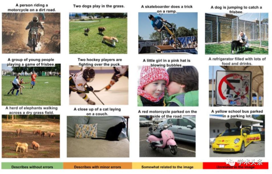Figure 1.6 Example of LSTM-generated captions, taken from “Show and Tell: A Neural Network Caption Generator”, 2014

1.5.2 Automatic Text Translation

The idea behind automatic text translation is to take sentences of text in one language and translate them into text in another language. For example, English sentences as input, and grammatical sentences as output. The model must learn the translation of words, modify the context of the translations, and support the lengths of input and output sequences that may vary overall.

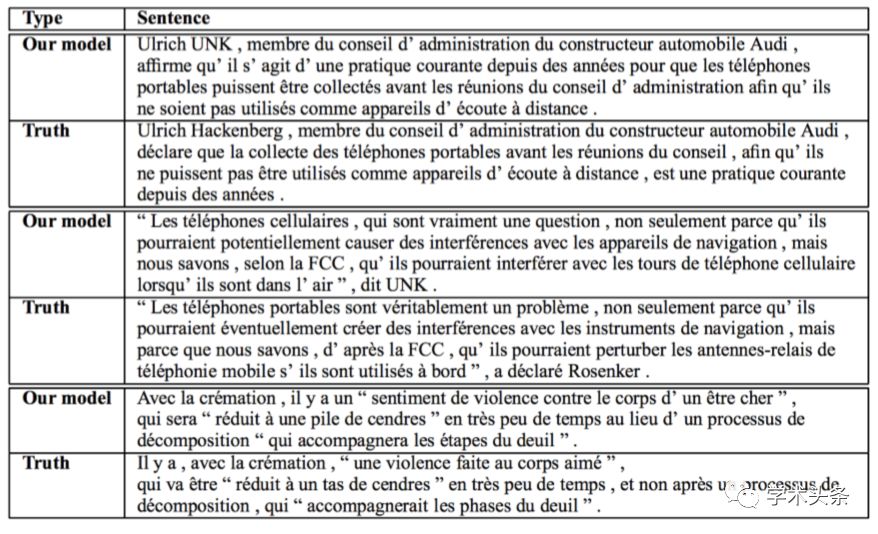Figure 1.7 Example of translating English text into French, from predictions to expected translations, taken from neural network sequence-to-sequence learning, 2014

1.5.3 Automatic Handwriting Generation

In this task, given a handwriting corpus, generate new handwriting for a given word or phrase. When handwriting samples are created, handwriting is provided as a sequence of coordinates used by the pen. In this corpus, the relationship between pen movements and letters is learned, producing new examples. Interestingly, different styles can be learned and then mimicked. I hope to see this work combined with some forensic handwriting analysis expertise. Figure 1.8 Example of LSTM-generated handwriting, taken from “Generating Sequences with Recurrent Neural Networks”, 2014

1.6 Limitations of LSTMs

LSTMs are impressive. The design of the network overcomes the technical challenges of RNNs and achieves guarantees for sequence prediction with neural networks. The applications of LSTMs have achieved impressive results on a range of complex problems. However, LSTMs may not be ideal for all sequence prediction problems.

For example, in time series prediction, it is often used to predict information within a small window of past observations. Typically, MLPs with windows or linear models may be a less complex and more suitable model.

Time series benchmark problems found in the literature… are often conceptually simpler than many tasks that LSTMs have already solved. They often do not require RNNs because all relevant information about the next event is conveyed by some recent events contained within a small time window.

— Applying LSTM to Time Series Predictable through Time-Window Approaches, 2001.

One important limitation of LSTMs is memory. Or more accurately, how memory can be abused. It is possible to force LSTM models to remember a single observation over long input time steps. This is a misuse of LSTMs, and requiring LSTM models to remember multiple observations will fail. When applying LSTMs to time series prediction, it can be seen that the problem is posed as regression, requiring removal as a function of multiple distant time steps in the input sequence. An LSTM might be forced to perform on this problem, but it is generally less than a well-designed autoregressive model or reconsidering the problem in general.

Assuming any dynamic model requires t-tau,… we note that [autoregression]-RNN must store all inputs from t-tau to t and cover them at the appropriate time. This requires implementing a cyclic cache, which is a structure that is very difficult to simulate for RNNs.

— Applying LSTM to Time Series Predictable through Time-Window Approaches, 2001.

Warning, LSTMs are not a new technology to be anticipated, and careful consideration of your problem framework is needed. Treat the internal state of LSTMs as a convenient internal variable to capture and provide context for predictions. If your problem looks like a traditional autoregressive problem, with the most relevant lags of observations within a small window, then perhaps using MLPs and sliding window development for performance baselines should be considered before considering LSTMs.

Time-window-based MLPs outperform pure-[autoregression] methods of LSTM on certain time series prediction benchmarks, simply by looking at a few recent inputs. Therefore, the special strength of LSTM, namely learning to remember individual events over long, positional time periods, is unnecessary.

— Applying LSTM to Time Series Predictable through Time-Window Approaches, 2001.

1.7 Further Reading

If you want to delve deeper into the technical details of the algorithms, here are some articles about LSTMs.

1.7.1 Sequence Prediction Problems

• Sequence on Wikipedia.

• On Prediction Using Variable Order Markov Models, 2004.

• Sequence Learning: From Recognition and Prediction to Sequential Decision Making, 2001.

• Chapter 14, Discrete Sequence Classification, Data Classification: Algorithms and Applications, 2015.

• Generating Sequences With Recurrent Neural Networks, 2013.

• Show and Tell: A Neural Image Caption Generator, 2015.

• Multi-task Sequence to Sequence Learning, 2016.

• Sequence to Sequence Learning with Neural Networks, 2014.

• Recursive and direct multi-step forecasting: the best of both worlds, 2012.

1.7.2 MLPs for Sequence Prediction

• Neural Networks for Time Series Processing, 1996.

• Sequence to Sequence Learning with Neural Networks, 2014.

1.7.3 Guarantees of RNNs

• Long Short-Term Memory Recurrent Neural Network Architectures for Large Scale Acoustic Modeling, 2014.

• Applying LSTM to Time Series Predictable through Time-Window Approaches, 2001.

• Long Short Term Memory Networks for Anomaly Detection in Time Series, 2015.

• Learning Long-Term Dependencies with Gradient Descent is Difficult, 1994.

• On the difficulty of training Recurrent Neural Networks, 2013.

1.7.4 LSTMs

• Long Short-Term Memory, 1997. Learning to forget: Continual prediction with LSTM, 2000.

• A Novel Connectionist System for Unconstrained Handwriting Recognition, 2009.

• Framewise Phoneme Classification with Bidirectional LSTM and Other Neural Network Architectures, 2005.

1.7.5 Applications of LSTMs

• Show and Tell: A Neural Image Caption Generator, 2014.

• Sequence to Sequence Learning with Neural Networks, 2014.

• Generating Sequences With Recurrent Neural Networks, 2014.

1.8 Expansion

1.9 Summary

In this lesson, you discovered Long Short-Term Memory Recurrent Neural Networks for sequence prediction. Did you know?

• What sequence prediction is? How does it differ from general predictive modeling problems?

• The limitations of Multilayer Perceptrons for sequence prediction, the guarantees of Recurrent Neural Networks for sequence prediction, and how LSTMs achieve that promise.

• Impressive applications of LSTMs that challenge sequence prediction problems, as well as some warnings about the limitations of LSTMs. Next, you will discover how to train LSTMs using backpropagation through time algorithms.

Author Introduction: Shao Zhou, PhD candidate. Research interests: data mining, scholar migration research.

(End)

More exciting:

46 people, the list of the world’s most cited scientists in computer science in mainland China in 2020!!!

[Yan Shi Series]: Intelligent Online Education Under the New Normal After the Epidemic

Heavy video benefits! 2020 Ideological Feast “Curriculum Ideology Face to Face” full set

Professor Li Xiaoming from Peking University: From Interesting Mathematics to Interesting Algorithms to Interesting Programming—A Path for Non-specialists to Experience Computational Thinking?

Several Thoughts on the Construction of First-class Computer Disciplines

Professor Liu Yunhao from Tsinghua University answers 2000 questions about AI

[Directory] “Computer Education” Issue 10, 2020

[Directory] “Computer Education” Issue 9, 2020

[Directory] “Computer Education” Issue 8, 2020

[Directory] “Computer Education” Issue 7, 2020

[Directory] “Computer Education” Issue 6, 2020

[Directory] “Computer Education” Issue 5, 2020

Professor Zhan Dechen from Harbin Institute of Technology: A New Model to Ensure Teaching Quality in Higher Education—Synchronous and Asynchronous Blended Teaching

Some Suggestions for Online Teaching—Li Fengxia from Beijing Institute of Technology

How should university teachers ensure the quality of online teaching? See what experts have to say

[Principal Interview] Accelerating the Advancement of Computer Science Education as a Pathfinder for Data Science Education—Interview with Professor Zhou Aoying, Vice President of East China Normal University

Editorial Message: From “Coffee on the Wall” to Computer Education

[Yan Shi Series] Analysis and Suggestions on the Quality Issues of Undergraduate Courses in Computer Majors

Analysis and Inspiration from the Computer Undergraduate Course Setup of the University of Tokyo, Japan

Teaching Reform and Practice of Artificial Intelligence Courses at Peking University

New Engineering and Big Data Major Construction

[Yan Shi Series] Distilling the Truth from the False—Starting from ESI Indicators

Learning from Others—Compilation of Research Articles on Computer Education at Home and Abroad