Click the image below to search【Interview Guide】 to obtain interview questions + resume templates.
In the field of machine learning, there is a saying that “there is no free lunch”. In simple terms, it means that no single algorithm can perform best on every problem. This theory is particularly important in supervised learning.
For example, you cannot say that neural networks are always better than decision trees, and vice versa. The performance of a model is influenced by many factors, such as the size and structure of the dataset.
Therefore, you should try many different algorithms based on your problem, while using a data test set to evaluate performance and select the best one.
Of course, the algorithms you try must be relevant to your problem, and this is the main task of machine learning. For example, if you want to clean your house, you might use a vacuum cleaner, a broom, or a mop, but you certainly wouldn’t start digging a hole with a shovel.
For those eager to understand the basics of machine learning, here is a list of the top ten machine learning algorithms used by data scientists, introducing the characteristics of these algorithms to help everyone better understand and apply them. Let’s take a look!
Linear regression is perhaps one of the most well-known and easiest to understand algorithms in statistics and machine learning.
Since predictive modeling primarily focuses on minimizing model error, or making the most accurate predictions at the cost of interpretability, we borrow, reuse, and steal algorithms from many different fields, which involves some statistical knowledge.
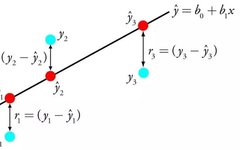
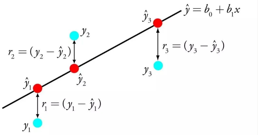
Linear regression is represented by an equation that describes the linear relationship between input variables (x) and output variables (y) by finding specific weights (B) for the input variables.
Given the input x, we will predict y, and the goal of the linear regression learning algorithm is to find the values of coefficients B0 and B1.
Different techniques can be used to learn the linear regression model from the data, such as linear algebra solutions for ordinary least squares and gradient descent optimization.
Linear regression has been around for over 200 years and has been extensively studied. Some rules of thumb when using this technique, if possible, are to remove very similar (correlated) variables and to remove noise from the data. This is a fast and simple technique and a good first algorithm to try.
Logistic regression is another technique borrowed from statistics in machine learning. It is a specialized method for binary classification problems (problems with two class values).
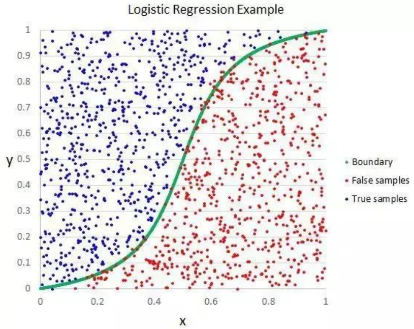
Logistic regression is similar to linear regression because both aim to find the weight values for each input variable. Unlike linear regression, however, the predicted output values are transformed using a nonlinear function called the logistic function.
The logistic function looks like a large S and can convert any value into a range between 0 and 1. This is useful because we can apply corresponding rules to the output of the logistic function, classifying values as 0 and 1 (for example, if IF less than 0.5, then output 1) and predicting class values.
Due to the unique learning method of the model, predictions made using logistic regression can also be used to calculate the probability of belonging to class 0 or class 1. This is very useful for problems that require providing many fundamental principles.
Like linear regression, logistic regression indeed performs better when you remove attributes that are unrelated to the output variable and attributes that are very similar (correlated) to each other. This is a quick-learning and efficient model for handling binary classification problems.
03 Linear Discriminant Analysis
Traditional logistic regression is limited to binary classification problems. If you have more than two classes, then Linear Discriminant Analysis (LDA) is the preferred linear classification technique.
LDA is very simply represented. It consists of the statistical properties of your data, calculated based on each class. For a single input variable, this includes:
-
-
The variance calculated across all classes.
LDA predicts by calculating the discriminant value for each class and predicting the class with the maximum value. This technique assumes that the data follows a Gaussian distribution (bell curve), so it is best to manually remove outliers from the data first. This is a simple yet powerful method for classification predictive modeling problems.
04 Classification and Regression Trees
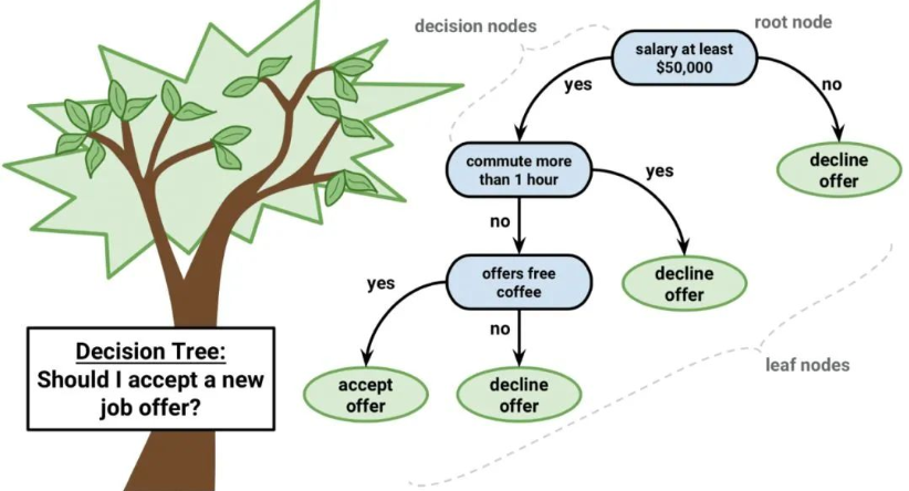
Decision trees are an important algorithm in machine learning.
Decision tree models can be represented as binary trees. Yes, a binary tree from algorithms and data structures, nothing special. Each node represents a single input variable (x) and the left and right children on that variable (assuming the variable is numeric).
The leaf nodes of the tree contain the output variable (y) used for making predictions. Predictions are made by traversing the tree, stopping when a leaf node is reached, and outputting the class value of that leaf node.
Decision trees are fast to learn and fast to predict. They often predict accurately for many problems, and you do not need to do any special preparation for the data.
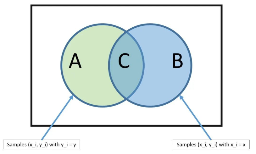
Naive Bayes is a simple yet extremely powerful predictive modeling algorithm.
The model consists of two types of probabilities that can be directly calculated from your training data: 1) the probability of each class; 2) the conditional probability of each x value given the class. Once calculated, the probability model can be used to predict new data using Bayes’ theorem. When your data is numerical, it is often assumed to follow a Gaussian distribution (bell curve) to easily estimate these probabilities.
Naive Bayes is called naive because it assumes that each input variable is independent. This is a tough assumption and unrealistic for real data, but the technique remains very effective for a wide range of complex problems.
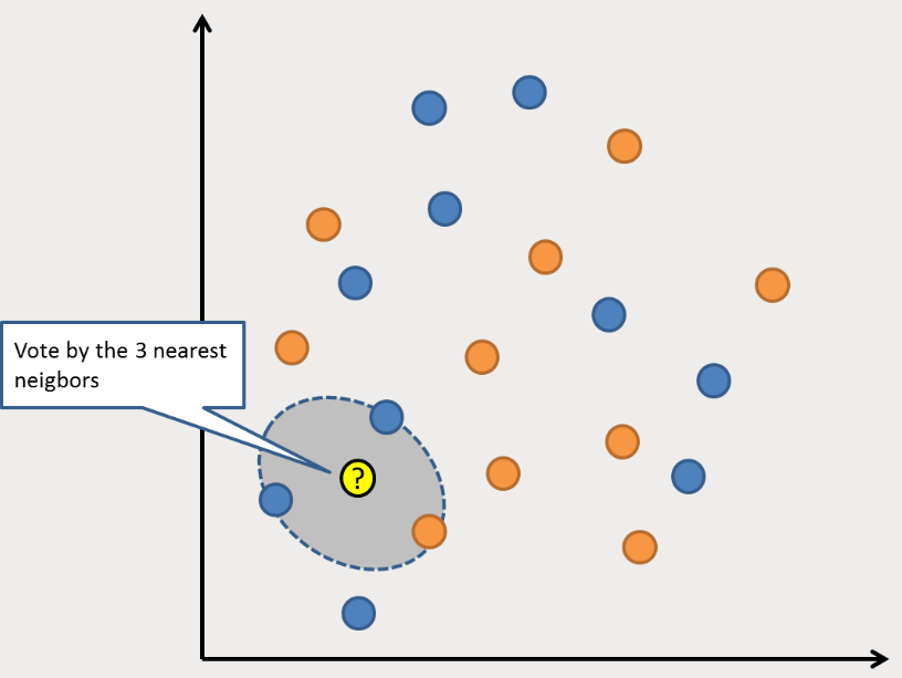
The KNN algorithm is very simple and very effective. The KNN model is represented by the entire training dataset. Isn’t that simple?
To predict a new data point, it searches the K most similar instances (neighbors) within the entire training set and aggregates the output variables of these K instances. For regression problems, the new point may be the average output variable, while for classification problems, the new point may be the mode class value.
The key to success lies in how to determine the similarity between data instances. If all your attributes are on the same scale, the simplest method is to use Euclidean distance, which can be directly calculated based on the distances between each input variable.
KNN may require a lot of memory or space to store all the data, but it only performs computations (or learning) when predictions are needed. You can also update and manage your training set at any time to maintain prediction accuracy.
The concept of distance or closeness may break down in high-dimensional environments (with many input variables), which can negatively impact the algorithm. Such events are referred to as the curse of dimensionality. It also implies that you should only use those input variables that are most relevant to the predicted output variable.
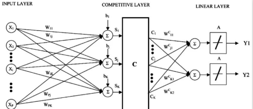
07 Learning Vector Quantization
The downside of K-Nearest Neighbors is that you need to maintain the entire training dataset. Learning Vector Quantization (or LVQ) is an artificial neural network algorithm that allows you to suspend any number of training instances and learn them accurately.
LVQ is represented by a set of codebook vectors. Initially, vectors are randomly chosen, and then iterated multiple times to adapt to the training dataset. After learning, codebook vectors can be used to predict just like K-Nearest Neighbors. By calculating the distance between each codebook vector and the new data instance, the most similar neighbor (best match) is found, and the class value of the best match unit or the actual value in the case of regression is returned as the prediction. You can achieve the best results if you keep the data within the same range (e.g., between 0 and 1).
If you find that KNN gives good results on your dataset, try using LVQ to reduce the memory requirements of storing the entire training dataset.
08 Support Vector Machines
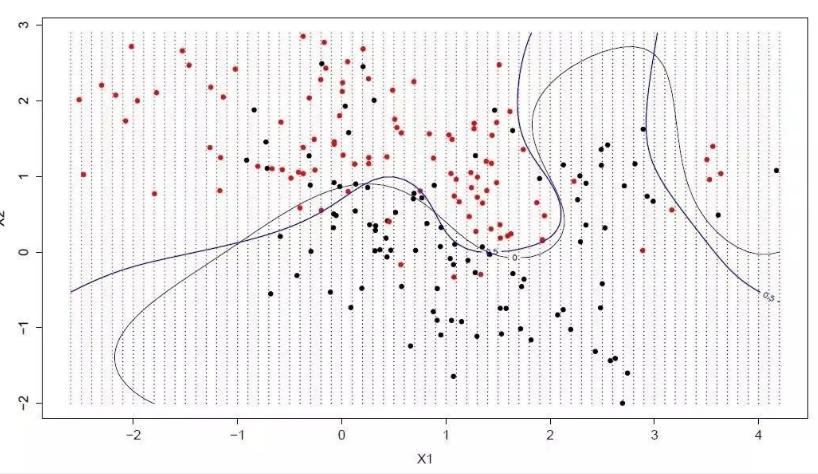
Support Vector Machines (SVM) may be one of the most popular and discussed machine learning algorithms.
A hyperplane is the line that divides the input variable space. In SVM, a hyperplane is chosen to separate points in the input variable space by their class (class 0 or class 1). In two-dimensional space, it can be viewed as a line that can completely separate all input points. The SVM learning algorithm aims to find the coefficient values that allow the hyperplane to best separate the classes.
The distance between the hyperplane and the nearest data points is called the margin, and the hyperplane with the maximum margin is the best choice. Furthermore, only those data points that are close to the hyperplane are relevant to its definition and the construction of the classifier; these points are called support vectors, which support or define the hyperplane. In practical applications, we use optimization algorithms to find the coefficient values that maximize the margin.
SVM may be one of the most powerful off-the-shelf classifiers and is worth trying on your dataset.
09 Bagging and Random Forests
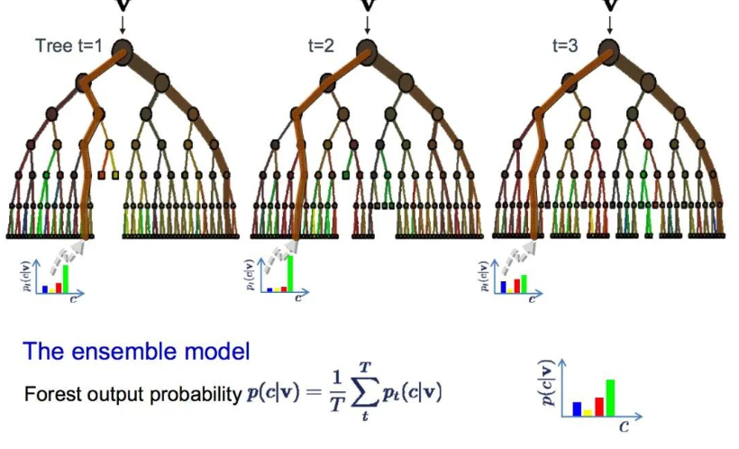
Random forests are one of the most popular and powerful machine learning algorithms. It is an ensemble machine learning algorithm known as Bootstrap Aggregation or Bagging.
Bootstrap is a powerful statistical method used to estimate a quantity, such as a mean, from a data sample. It draws many samples from the data, calculates the mean, and averages all the means to more accurately estimate the true mean.
In bagging, the same method is used, but the most commonly used model is the decision tree, rather than estimating an entire statistical model. It trains the data through multiple sampling and builds a model for each data sample. When you need to predict new data, each model makes predictions, and the predicted results are averaged to better estimate the true output value.
Random forests are a modification of decision trees, where randomization is introduced to achieve suboptimal splits instead of selecting the best split point.
Thus, the variability between the models created for each data sample will be greater, but still accurate in its own right. Combining the prediction results can better estimate the correct potential output values.
If you achieve good results with high variance algorithms (like decision trees), adding this algorithm will improve the results further.
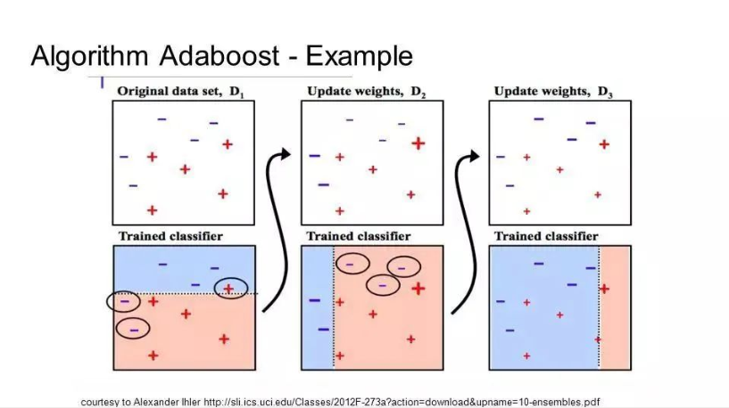
Boosting is an ensemble technique that creates a strong classifier from several weak classifiers. It first builds a model from the training data and then creates a second model to try to correct the errors of the first model. Models are added continuously until the training set is perfectly predicted or the maximum number has been reached.
AdaBoost is the first truly successful boosting algorithm developed for binary classification and is the best starting point for understanding boosting. The most famous algorithms built on AdaBoost are currently gradient boosting.
AdaBoost is often used with short decision trees. After creating the first tree, the performance of each training instance on the tree determines how much attention the next tree needs to pay to this training instance. Hard-to-predict training data will be given more weight, while easily predicted instances will be given less weight. Models are created sequentially, and the updates of each model affect the learning of the next tree in the sequence. After all trees are built, the algorithm predicts new data and weights the performance of each tree based on the accuracy of the training data.
Because the algorithm places great emphasis on error correction, it is crucial to have clean data without outliers.
A typical question that beginners ask when faced with various machine learning algorithms is, “Which algorithm should I use?” The answer to this question depends on many factors, including:
-
The size, quality, and nature of the data;
-
The available computation time;
-
-
What you want to do with the data.
Even an experienced data scientist cannot know which algorithm will perform best without trying different ones. While there are many other machine learning algorithms, these are the most popular. If you are new to machine learning, this is a great starting point for learning.
Recent Courses Available:
Common Data Structures | Excel Basics | Database Operations | Scrapy Framework | Numpy | SQL Structured Query Language | Data Analysis Practice | Object-Oriented Programming | Project Practice | Matplotlib
We recommend a highly-rated Python learning mini-program「Qianfeng Learning Station」.
Click the card below to start learning