Produced by Big Data Digest

Compiled by: Hong Yingfei, Ning Jing

PyTorch is one of the deep learning framework libraries, an open-source deep learning platform from Facebook, providing seamless connection from research prototype to production deployment.

This article aims to introduce the basics of PyTorch, helping beginners write their first Python PyTorch code in 4 minutes.

All the functional functions mentioned below can be viewed in detail in the Chinese documentation, here is the link to the PyTorch Chinese documentation:

https://pytorch-cn.readthedocs.io/zh/latest/package_references/torch/

Preparation Before Coding

You need to install the Python package on your computer and import some scientific computing packages, such as: numpy, etc. The most important thing is to remember to import PyTorch. The results below are obtained in Jupyter Notebook, interested readers can download Anaconda, which comes with Jupyter Notebook. (Note: Anaconda supports multiple versions of Python virtual compilation environments, Jupyter Notebook is a web-based compilation interface that splits code into cells, allowing real-time viewing of running results, very convenient to use!)

There are many tutorials online for software configuration and installation, so I won’t elaborate here. Knowledge gained from books is shallow; real understanding comes from practice. Let’s directly enter the world of PyTorch and start coding!

Tensors

The Tensor class is an important fundamental data type in neural network frameworks, which can be simply understood as a multi-dimensional matrix containing elements of a single data type. Tensors are connected through operations to form a computation graph.

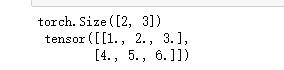
The following code example creates a 2×3 2D tensor x, specifying the data type as float:

import torch
# Tensors
x = torch.FloatTensor([[1, 2, 3], [4, 5, 6]])
print(x.size(), "\n", x)

Running result:

PyTorch includes many mathematical operations on tensors. In addition, it provides many utilities, such as efficient serialization of Tensors and other arbitrary data types, as well as other useful utilities.

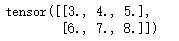
Below is an example of tensor addition/subtraction, where torch.ones(*sizes, out=None) → Tensor returns a tensor filled with ones, with the shape defined by the variable parameter sizes. In this example, x is added to two 2×3 tensors with corresponding positions set to 1, which is equivalent to adding 2 to the value of each dimension of x. The code and running results are as follows:

# Add tensors
x.add_(torch.ones([2, 3]) + torch.ones([2, 3]))

Running result:

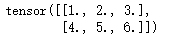
Similarly, PyTorch also supports subtraction operations, as shown below, where 2 is subtracted from each dimension based on the previous running result, restoring x to its original value.

# Subtract Tensor
x.sub_(torch.ones([2, 3]) * 2)

Running result:

Other PyTorch operations can be found in the Chinese link provided above.

PyTorch and NumPy

Users can easily convert between PyTorch and NumPy.

Below is a simple example of converting a np.matrix to PyTorch and changing its dimension to a single column:

# Numpy to torch tensors
import numpy as np

y = np.matrix([[2, 2], [2, 2], [2, 2]])
z = np.matrix([[2, 2], [2, 2], [2, 2]], dtype="int16")
x.short() @ torch.from_numpy(z)

Running result:

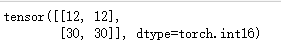
Where @ is the overloaded operator for tensor multiplication, x is a 2×3 tensor with values [[1, 2, 3], [4, 5, 6]], multiplied by the converted tensor z, which is of size 3×2, resulting in a 2×2 tensor. (Similar to matrix multiplication; readers who do not understand the running results can refer to matrix multiplication operations)

Additionally, PyTorch also supports tensor structure reshaping, below is an example of reshaping tensor x into a 1×6 one-dimensional tensor, similar to the reshape function in numpy.

# Reshape tensors (similar to np.reshape)
x.view(1, 6)

Running result:

GitHub repo outlines the conversion from PyTorch to numpy, link as follows:

https://github.com/wkentaro/pytorch-for-numpy-users

CPU and GPUs

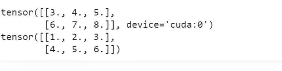
PyTorch allows variables to dynamically change devices using the torch.cuda.device context manager. Below is sample code:

# move variables and copies across computer devices
x = torch.FloatTensor([[1, 2, 3], [4, 5, 6]])
y = np.matrix([[2, 2, 2], [2, 2, 2]], dtype="float32")

if(torch.cuda.is_available()):
    x = x.cuda();
    y = torch.from_numpy(y).cuda()
    z = x + y
print(z)
print(x.cpu())

Running result:

PyTorch Variables

Variables are just thin wrappers around Tensors that support almost all APIs defined by Tensors. Variables are cleverly defined as part of the automatic differentiation package. They provide classes and functions for automatic differentiation of any scalar-valued functions.

Below is a simple example of using PyTorch variables, where the result of multiplying v1 and v2 is assigned to v3. The requires_grad attribute of the parameter inside is set to False by default. If a node’s requires_grad is set to True, then all nodes depending on it will also have requires_grad set to True, primarily used for gradient computation.

# Variable (part of autograd package)
# Variable (graph nodes) are thin wrappers around tensors and have dependency knowledge
# Variable enables backpropagation of gradients and automatic differentiations
# Variable are set a 'volatile' flag during inference

from torch.autograd import Variable
v1 = Variable(torch.tensor([1., 2., 3.]), requires_grad=False)
v2 = Variable(torch.tensor([4., 5., 6.]), requires_grad=True)
v3 = v1 * v2

v3.data.numpy()

Running result:

# Variables remember what created them
v3.grad_fn

Running result:

Back Propagation

The backpropagation algorithm is used to compute the loss gradient with respect to input weights and biases to update the weights in the next optimization iteration and ultimately reduce the loss. PyTorch is very smart in defining the backward method for variables to perform backpropagation.

Below is a simple method for backpropagation calculation, using sin(x) as an example to compute the difference:

# Backpropagation with example of sin(x)
x = Variable(torch.Tensor(np.array([0., 1., 1.5, 2.]) * np.pi), requires_grad=True)
y = torch.sin(x)
x.grad.backward(torch.Tensor([1., 1., 1., 1]))

# Check gradient is indeed cos(x)
if((x.grad.data.int().numpy() == torch.cos(x).data.int().numpy()).all()):
    print("d(sin(x)/dx=cos(x))")

Running result:

For variables and gradient computation in PyTorch, you can refer to the article below:

https://zhuanlan.zhihu.com/p/29904755

SLR: Simple Linear Regression

Now that we understand the basics, we can start using PyTorch to solve simple machine learning problems—simple linear regression. We will complete it in 4 simple steps:

Step One

In step 1, we create a synthetic dataset generated by the equation y = wx + b, injecting random errors. See the example below:

# Simple Linear Regression
# Fit a line to the data. Y = w.x + b
# Deterministic behavior
np.random.seed(0)
torch.manual_seed(0)
# Step 1: Dataset
w = 2;
b = 3
x = np.linspace(0, 10, 100)
y = w * x + b + np.random.randn(100) * 2
x = x.reshape(-1, 1)
y = y.reshape(-1, 1)

In step 2, we define a simple class LinearRegressionModel using the forward function, and use torch.nn.Linear to define the constructor for linear transformation of the input data:

# Step 2: Model
class LinearRegressionModel(torch.nn.Module):
    def __init__(self, in_dimn, out_dimn):
        super(LinearRegressionModel, self).__init__()
        self.model = torch.nn.Linear(in_dimn, out_dimn)

    def forward(self, x):
        y_pred = self.model(x);
        return y_pred;

model = LinearRegressionModel(in_dimn=1, out_dimn=1)

Reference for torch.nn.Linear:

https://pytorch.org/docs/stable/_modules/torch/nn/modules/linear.html

Step Three

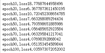
The next step: use MSELoss as the cost function and SGD as the optimizer to train the model.

# Step 3: Training
cost = torch.nn.MSELoss()
optimizer = torch.optim.SGD(model.parameters(), lr=0.01, momentum=0.9)
inputs = Variable(torch.from_numpy(x.astype("float32")))
outputs = Variable(torch.from_numpy(y.astype("float32")))

for epoch in range(100):
    # 3.1 forward pass:
    y_pred = model(inputs)
    # 3.2 compute loss
    loss = cost(y_pred, outputs)
    # 3.3 backward pass
    optimizer.zero_grad();
    loss.backward()
    optimizer.step()
    if((epoch + 1) % 10 == 0):
        print("epoch {}, loss {}".format(epoch + 1, loss.data))

Running result:

Reference for MSELoss:

https://pytorch.org/docs/stable/_modules/torch/nn/modules/loss.html

Reference for SGD:

https://pytorch.org/docs/stable/_modules/torch/optim/sgd.html

Step Four

Now that training is complete, let’s visually check our model:

# Step 4: Display model and confirm
import matplotlib.pyplot as plt
plt.figure(figsize=(4, 4))
plt.title("Model and Dataset")
plt.xlabel("X");
plt.ylabel("Y")
plt.grid()
plt.plot(x, y, "ro", label="DataSet", marker="x", markersize=4)
plt.plot(x, model.model.weight.item() * x + model.model.bias.item(), label="Regression Model")
plt.legend();
plt.show()

Running result:

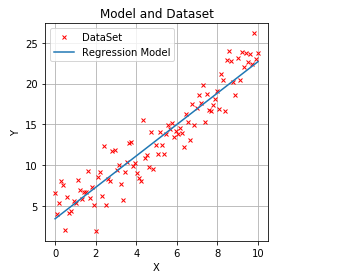
Now you have completed the programming of your first linear regression example in PyTorch. For readers who wish to further enhance their skills, you can refer to the official PyTorch documentation link to complete most coding applications.

Related links:

https://medium.com/towards-artificial-intelligence/pytorch-in-2-minutes-9e18875990fd

Exciting! The Academic WeChat Group for Natural Language Processing has been established

You can scan the QR code below to join the group for communication,

Note: Please modify the remark as [School/Company + Name + Direction] when adding

For example — Harbin Institute of Technology + Zhang San + Dialogue System.

Account owner, please avoid business promotion. Thank you!

Recommended Reading:
【Detailed Explanation】From Transformer to BERT Model
Sai Er Translation | Understanding Transformer from Scratch
Seeing is better than hearing! A step-by-step guide to building a Transformer with Python