
Click the "Xiaobai Learns Vision" above, choose to add "Star" or "Top"

Heavyweight content delivered at the first time
Author丨Jiefa Shouzhangsheng@Zhihu
Link丨https://zhuanlan.zhihu.com/p/559887437
Using data augmentation techniques can increase the diversity of images in the dataset, thereby improving the performance and generalization ability of the model. The main image augmentation techniques include:
-
Resize -
Grayscale Transformation -
Normalization -
Random Rotation -
Center Crop -
Random Crop -
Gaussian Blur -
Brightness and Contrast Adjustment -
Horizontal Flip -
Vertical Flip -
Gaussian Noise -
Random Blocks -
Central Region
Resize
Before resizing the image, we need to import the data (taking fundus images as an example).
from PIL import Image
from pathlib import Path
import matplotlib.pyplot as plt
import numpy as np
import sys
import torch
import numpy as np
import torchvision.transforms as T

plt.rcParams["savefig.bbox"] = 'tight'
orig_img = Image.open(Path('image/000001.tif'))
torch.manual_seed(0) # Set the seed for generating random numbers on CPU for reproducibility
print(np.asarray(orig_img).shape) #(800, 800, 3)

# Resize the image
resized_imgs = [T.Resize(size=size)(orig_img) for size in [128,256]]
# plt.figure('resize:128*128')
ax1 = plt.subplot(131)
ax1.set_title('original')
ax1.imshow(orig_img)

ax2 = plt.subplot(132)
ax2.set_title('resize:128*128')
ax2.imshow(resized_imgs[0])

ax3 = plt.subplot(133)
ax3.set_title('resize:256*256')
ax3.imshow(resized_imgs[1])

plt.show()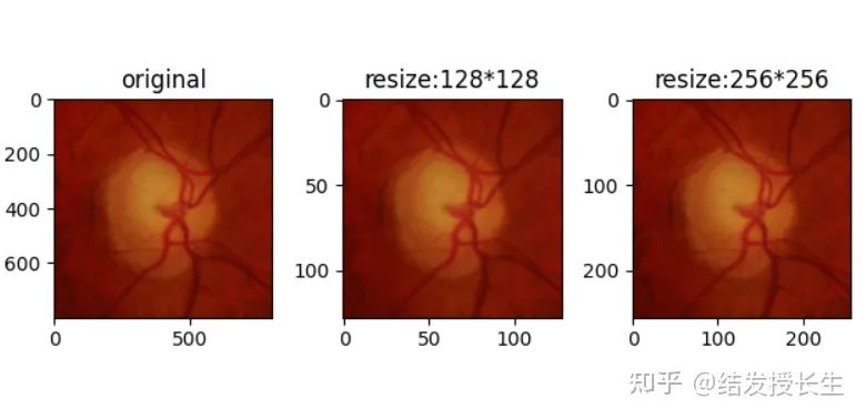
Grayscale Transformation
This operation converts an RGB image to a grayscale image.
gray_img = T.Grayscale()(orig_img)
# plt.figure('resize:128*128')
ax1 = plt.subplot(121)
ax1.set_title('original')
ax1.imshow(orig_img)

ax2 = plt.subplot(122)
ax2.set_title('gray')
ax2.imshow(gray_img,cmap='gray')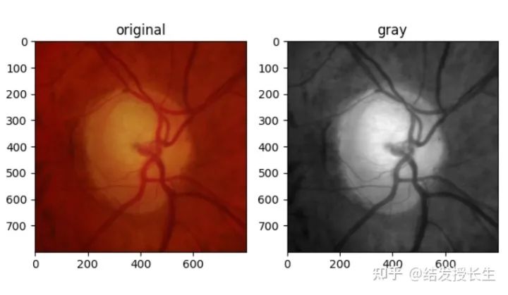
Normalization
Normalization can accelerate the computation speed of models based on neural network structures and speed up the learning process.
-
Subtract the channel mean from each input channel -
Divide by the channel standard deviation.
normalized_img = T.Normalize(mean=(0.5, 0.5, 0.5), std=(0.5, 0.5, 0.5))(T.ToTensor()(orig_img))
normalized_img = [T.ToPILImage()(normalized_img)]
# plt.figure('resize:128*128')
ax1 = plt.subplot(121)
ax1.set_title('original')
ax1.imshow(orig_img)

ax2 = plt.subplot(122)
ax2.set_title('normalize')
ax2.imshow(normalized_img[0])

plt.show()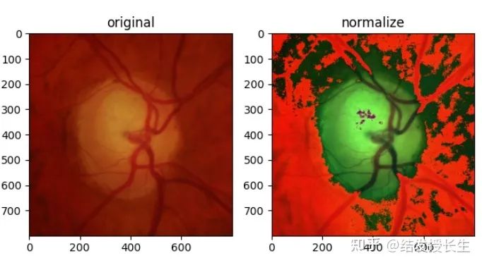
Random Rotation
Rotate the image at a designed angle
from PIL import Image
from pathlib import Path
import matplotlib.pyplot as plt
import numpy as np
import sys
import torch
import numpy as np
import torchvision.transforms as T

plt.rcParams["savefig.bbox"] = 'tight'
orig_img = Image.open(Path('image/2.png'))

rotated_imgs = [T.RandomRotation(degrees=90)(orig_img)]
print(rotated_imgs)
plt.figure('resize:128*128')
ax1 = plt.subplot(121)
ax1.set_title('original')
ax1.imshow(orig_img)

ax2 = plt.subplot(122)
ax2.set_title('90°')
ax2.imshow(np.array(rotated_imgs[0]))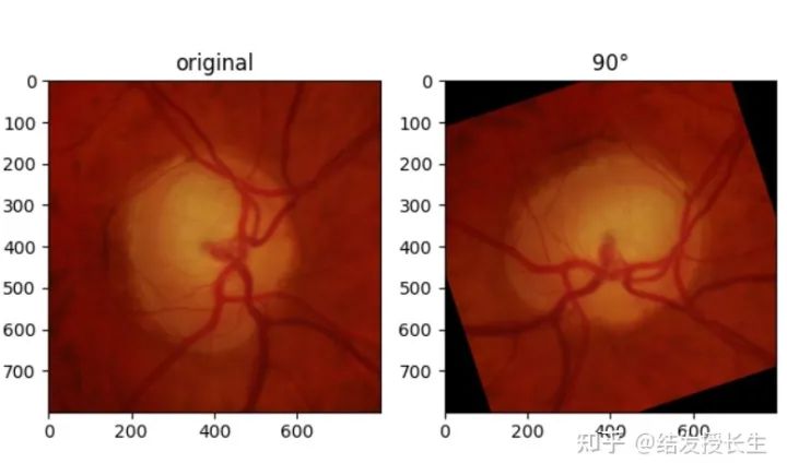
Center Crop
Crop the center region of the image
from PIL import Image
from pathlib import Path
import matplotlib.pyplot as plt
import numpy as np
import sys
import torch
import numpy as np
import torchvision.transforms as T

plt.rcParams["savefig.bbox"] = 'tight'
orig_img = Image.open(Path('image/2.png'))

center_crops = [T.CenterCrop(size=size)(orig_img) for size in (128,64)]

plt.figure('resize:128*128')
ax1 = plt.subplot(131)
ax1.set_title('original')
ax1.imshow(orig_img)

ax2 = plt.subplot(132)
ax2.set_title('128*128°')
ax2.imshow(np.array(center_crops[0]))

ax3 = plt.subplot(133)
ax3.set_title('64*64')
ax3.imshow(np.array(center_crops[1]))

plt.show()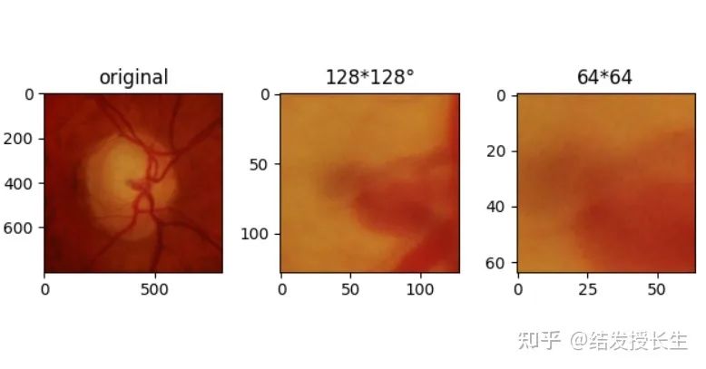
Random Crop
Randomly crop a part of the image
from PIL import Image
from pathlib import Path
import matplotlib.pyplot as plt
import numpy as np
import sys
import torch
import numpy as np
import torchvision.transforms as T

plt.rcParams["savefig.bbox"] = 'tight'
orig_img = Image.open(Path('image/2.png'))

random_crops = [T.RandomCrop(size=size)(orig_img) for size in (400,300)]

plt.figure('resize:128*128')
ax1 = plt.subplot(131)
ax1.set_title('original')
ax1.imshow(orig_img)

ax2 = plt.subplot(132)
ax2.set_title('400*400')
ax2.imshow(np.array(random_crops[0]))

ax3 = plt.subplot(133)
ax3.set_title('300*300')
ax3.imshow(np.array(random_crops[1]))

plt.show()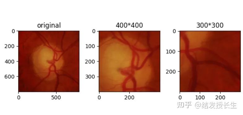
Gaussian Blur
Use a Gaussian kernel to blur the image
from PIL import Image
from pathlib import Path
import matplotlib.pyplot as plt
import numpy as np
import sys
import torch
import numpy as np
import torchvision.transforms as T

plt.rcParams["savefig.bbox"] = 'tight'
orig_img = Image.open(Path('image/2.png'))

blurred_imgs = [T.GaussianBlur(kernel_size=(3, 3), sigma=sigma)(orig_img) for sigma in (3,7)]

plt.figure('resize:128*128')
ax1 = plt.subplot(131)
ax1.set_title('original')
ax1.imshow(orig_img)

ax2 = plt.subplot(132)
ax2.set_title('sigma=3')
ax2.imshow(np.array(blurred_imgs[0]))

ax3 = plt.subplot(133)
ax3.set_title('sigma=7')
ax3.imshow(np.array(blurred_imgs[1]))

plt.show()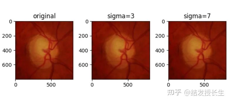
Brightness, Contrast, and Saturation Adjustment
from PIL import Image
from pathlib import Path
import matplotlib.pyplot as plt
import numpy as np
import sys
import torch
import numpy as np
import torchvision.transforms as T

plt.rcParams["savefig.bbox"] = 'tight'
orig_img = Image.open(Path('image/2.png'))
# random_crops = [T.RandomCrop(size=size)(orig_img) for size in (832,704, 256)]
colorjitter_img = [T.ColorJitter(brightness=(2,2), contrast=(0.5,0.5), saturation=(0.5,0.5))(orig_img)]

plt.figure('resize:128*128')
ax1 = plt.subplot(121)
ax1.set_title('original')
ax1.imshow(orig_img)
ax2 = plt.subplot(122)
ax2.set_title('colorjitter_img')
ax2.imshow(np.array(colorjitter_img[0]))
plt.show()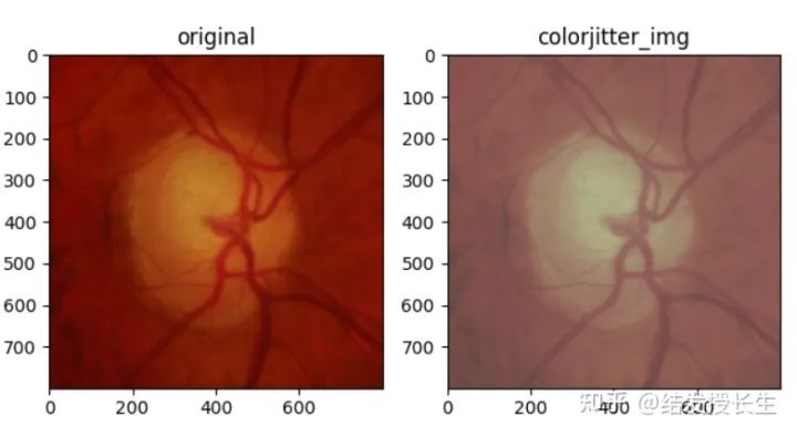
Horizontal Flip
from PIL import Image
from pathlib import Path
import matplotlib.pyplot as plt
import numpy as np
import sys
import torch
import numpy as np
import torchvision.transforms as T

plt.rcParams["savefig.bbox"] = 'tight'
orig_img = Image.open(Path('image/2.png'))

HorizontalFlip_img = [T.RandomHorizontalFlip(p=1)(orig_img)]

plt.figure('resize:128*128')
ax1 = plt.subplot(121)
ax1.set_title('original')
ax1.imshow(orig_img)

ax2 = plt.subplot(122)
ax2.set_title('colorjitter_img')
ax2.imshow(np.array(HorizontalFlip_img[0]))

plt.show()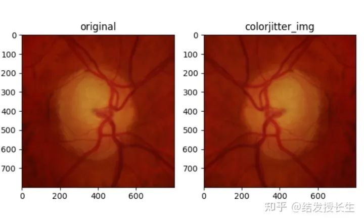
Vertical Flip
from PIL import Image
from pathlib import Path
import matplotlib.pyplot as plt
import numpy as np
import sys
import torch
import numpy as np
import torchvision.transforms as T

plt.rcParams["savefig.bbox"] = 'tight'
orig_img = Image.open(Path('image/2.png'))

VerticalFlip_img = [T.RandomVerticalFlip(p=1)(orig_img)]

plt.figure('resize:128*128')
ax1 = plt.subplot(121)
ax1.set_title('original')
ax1.imshow(orig_img)

ax2 = plt.subplot(122)
ax2.set_title('VerticalFlip')
ax2.imshow(np.array(VerticalFlip_img[0]))

# ax3 = plt.subplot(133)
# ax3.set_title('sigma=7')
# ax3.imshow(np.array(blurred_imgs[1]))

plt.show()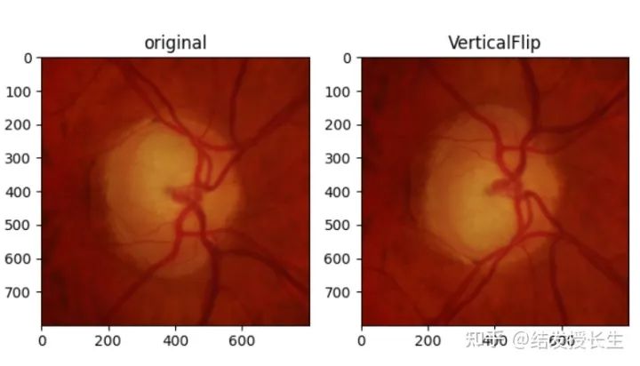
Gaussian Noise
Add Gaussian noise to the image. The higher the noise factor, the greater the noise in the image.
from PIL import Image
from pathlib import Path
import matplotlib.pyplot as plt
import numpy as np
import sys
import torch
import numpy as np
import torchvision.transforms as T

plt.rcParams["savefig.bbox"] = 'tight'
orig_img = Image.open(Path('image/2.png'))

def add_noise(inputs, noise_factor=0.3):
    noisy = inputs + torch.randn_like(inputs) * noise_factor
    noisy = torch.clip(noisy, 0., 1.)
    return noisy

noise_imgs = [add_noise(T.ToTensor()(orig_img), noise_factor) for noise_factor in (0.3, 0.6)]
noise_imgs = [T.ToPILImage()(noise_img) for noise_img in noise_imgs]

plt.figure('resize:128*128')
ax1 = plt.subplot(131)
ax1.set_title('original')
ax1.imshow(orig_img)

ax2 = plt.subplot(132)
ax2.set_title('noise_factor=0.3')
ax2.imshow(np.array(noise_imgs[0]))

ax3 = plt.subplot(133)
ax3.set_title('noise_factor=0.6')
ax3.imshow(np.array(noise_imgs[1]))

plt.show()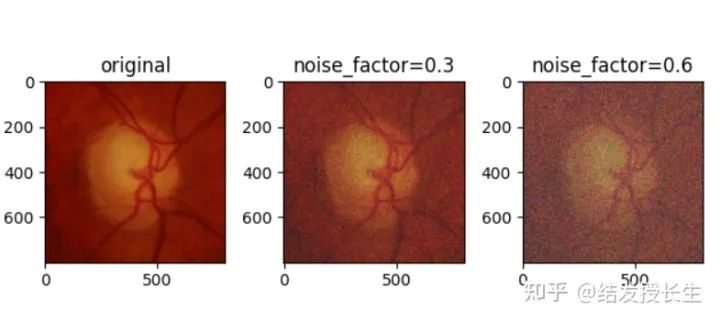
Random Blocks
Randomly apply square patches to the image. The more patches, the harder it is for the neural network to solve the problem.
from PIL import Image
from pathlib import Path
import matplotlib.pyplot as plt
import numpy as np
import sys
import torch
import numpy as np
import torchvision.transforms as T

plt.rcParams["savefig.bbox"] = 'tight'
orig_img = Image.open(Path('image/2.png'))

def add_random_boxes(img,n_k,size=64):
    h,w = size,size
    img = np.asarray(img).copy()
    img_size = img.shape[1]
    boxes = []
    for k in range(n_k):
        y,x = np.random.randint(0,img_size-w,(2,))
        img[y:y+h,x:x+w] = 0
        boxes.append((x,y,h,w))
    img = Image.fromarray(img.astype('uint8'), 'RGB')
    return img

blocks_imgs = [add_random_boxes(orig_img,n_k=10)]

plt.figure('resize:128*128')
ax1 = plt.subplot(131)
ax1.set_title('original')
ax1.imshow(orig_img)

ax2 = plt.subplot(132)
ax2.set_title('10 black boxes')
ax2.imshow(np.array(blocks_imgs[0]))

plt.show()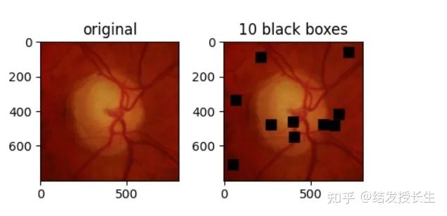
Central Region
Similar to random blocks, but patches are added in the center of the image
from PIL import Image
from pathlib import Path
import matplotlib.pyplot as plt
import numpy as np
import sys
import torch
import numpy as np
import torchvision.transforms as T

plt.rcParams["savefig.bbox"] = 'tight'
orig_img = Image.open(Path('image/2.png'))

def add_central_region(img, size=32):
    h, w = size, size
    img = np.asarray(img).copy()
    img_size = img.shape[1]
    img[int(img_size / 2 - h):int(img_size / 2 + h), int(img_size / 2 - w):int(img_size / 2 + w)] = 0
    img = Image.fromarray(img.astype('uint8'), 'RGB')
    return img

central_imgs = [add_central_region(orig_img, size=128)]

plt.figure('resize:128*128')
ax1 = plt.subplot(131)
ax1.set_title('original')
ax1.imshow(orig_img)

ax2 = plt.subplot(132)
ax2.set_title('')
ax2.imshow(np.array(central_imgs[0]))
#
# ax3 = plt.subplot(133)
# ax3.set_title('20 black boxes')
# ax3.imshow(np.array(blocks_imgs[1]))

plt.show()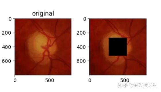
Download 1: OpenCV-Contrib Extension Module Chinese Version Tutorial

Reply "Extension Module Chinese Tutorial" in the "Xiaobai Learns Vision" public account backstage to download the first OpenCV extension module tutorial in Chinese, covering installation of extension modules, SFM algorithms, stereo vision, object tracking, biological vision, super-resolution processing, and more than twenty chapters of content.

Download 2: Python Vision Practical Project 52 Lectures

Reply "Python Vision Practical Project" in the "Xiaobai Learns Vision" public account backstage to download 31 practical vision projects including image segmentation, mask detection, lane line detection, vehicle counting, adding eyeliner, license plate recognition, character recognition, emotion detection, text content extraction, facial recognition, etc., to assist in quickly learning computer vision.

Download 3: OpenCV Practical Projects 20 Lectures

Reply "OpenCV Practical Projects 20 Lectures" in the "Xiaobai Learns Vision" public account backstage to download 20 practical projects based on OpenCV, achieving advanced learning of OpenCV.

Communication Group

Welcome to join the public account reader group to exchange with peers. Currently, there are WeChat groups for SLAM, 3D vision, sensors, autonomous driving, computational photography, detection, segmentation, recognition, medical imaging, GAN, algorithm competitions, etc. (will gradually be subdivided in the future). Please scan the WeChat account below to join the group, and note: "Nickname + School/Company + Research Direction", for example: "Zhang San + Shanghai Jiao Tong University + Visual SLAM". Please follow the format, otherwise it will not be approved. After successfully adding, you will be invited into the relevant WeChat group based on your research direction. Please do not send advertisements in the group, otherwise you will be asked to leave the group. Thank you for your understanding~