Illustrated Machine Learning Practice showcases the application process and the various stages of machine learning algorithms through case studies and code, enabling the mastery of building scenario modeling solutions and optimizing performance.

This article provides a detailed explanation of the engineering application methods of XGBoost. XGBoost is a powerful boosting algorithm toolkit and is the model of choice for many major companies’ machine learning solutions, excelling in parallel computing efficiency, handling missing values, and controlling overfitting.

https://www.showmeai.tech/article-detail/204

XGBoost stands for eXtreme Gradient Boosting, which is a very powerful boosting algorithm toolkit. Its excellent performance (both effectiveness and speed) has kept it at the top of data science competition solutions for a long time. Many major companies still prefer this model in their machine learning solutions. XGBoost performs exceptionally well in parallel computing efficiency, handling missing values, controlling overfitting, and generalization capability.

This content is presented by ShowMeAI, explaining the engineering application methods of XGBoost. Students interested in the principles of XGBoost are welcome to refer to another article by ShowMeAI: Illustrated Machine Learning | Detailed Explanation of XGBoost Model^[1].

1. Installing XGBoost

XGBoost, as a common and powerful Python machine learning library, is relatively simple to install.

Setting Up Python and IDE Environment

For setting up the Python environment and IDE, you can refer to the ShowMeAI article Illustrated Python | Installation and Environment Setup^[2].

Installing the Toolkit

(1) Linux/Mac and Other Systems

For installing XGBoost on these systems, you can easily complete it using pip. Just enter the following command in the command line and wait for the installation to finish.

pip install xgboost

You can also choose a domestic pip source for better installation speed.

pip install -i https://pypi.tuna.tsinghua.edu.cn/simple xgboost

(2) Windows System

For Windows systems, a more efficient and convenient installation method is to download the corresponding version of the XGBoost installation package from the website http://www.lfd.uci.edu/~gohlke/pythonlibs/ and then install it using the following command.

pip install xgboost‑1.5.1‑cp310‑cp310‑win32.whl

2. Reading Data with XGBoost

The first step in using XGBoost is to load the required data into a format supported by the toolkit. XGBoost can load various data formats for training modeling:

The SKLearn interface of XGBoost also supports processing data in DataFrame format (for more information, refer to ShowMeAI’s article Python Data Analysis | Comprehensive Core Operations of Pandas^[3]).

Below are different formats of data and the loading methods in XGBoost.

dtrain1 = xgb.DMatrix('train.svm.txt')

dtrain2 = xgb.DMatrix('train.svm.buffer')

data = np.random.rand(5,10) # 5 entities, each contains 10 features
label = np.random.randint(2, size=5) # binary target
dtrain = xgb.DMatrix( data, label=label)

csr = scipy.sparse.csr_matrix( (dat, (row,col)) )
dtrain = xgb.DMatrix( csr )

dtrain = xgb.DMatrix('train.svm.txt')
dtrain.save_binary("train.buffer")

dtrain = xgb.DMatrix( data, label=label, missing = -999.0)

w = np.random.rand(5,1)
dtrain = xgb.DMatrix( data, label=label, missing = -999.0, weight=w)

3. Different Modeling Methods of XGBoost

Built-in Modeling Method: libsvm Format Data Source

XGBoost has built-in modeling methods with the following data formats and core training methods:

Below is a simple example from the official documentation that demonstrates the process of reading libsvm format data (into DMatrix format) and specifying parameters for modeling.

# Import the toolkit
import numpy as np
import scipy.sparse
import pickle
import xgboost as xgb

# Read data from libsvm file for binary classification
# The data is in libsvm format, as shown below:
#1 3:1 10:1 11:1 21:1 30:1 34:1 36:1 40:1 41:1 53:1 58:1 65:1 69:1 77:1 86:1 88:1 92:1 95:1 102:1 105:1 117:1 124:1
#0 3:1 10:1 20:1 21:1 23:1 34:1 36:1 39:1 41:1 53:1 56:1 65:1 69:1 77:1 86:1 88:1 92:1 95:1 102:1 106:1 116:1 120:1
#0 1:1 10:1 19:1 21:1 24:1 34:1 36:1 39:1 42:1 53:1 56:1 65:1 69:1 77:1 86:1 88:1 92:1 95:1 102:1 106:1 116:1 122:1
dtrain = xgb.DMatrix('./data/agaricus.txt.train')
dtest = xgb.DMatrix('./data/agaricus.txt.test')

# Set hyperparameters
# Mainly tree depth, learning rate, objective function
param = {'max_depth':2, 'eta':1, 'silent':1, 'objective':'binary:logistic' }

# Set watchlist to observe model status during training
watchlist  = [(dtest,'eval'), (dtrain,'train')]
num_round = 2
bst = xgb.train(param, dtrain, num_round, watchlist)

# Use the model for prediction
preds = bst.predict(dtest)

# Calculate accuracy
labels = dtest.get_label()
print('Error rate is %f' % 
       (sum(1 for i in range(len(preds)) if int(preds[i]>0.5)!=labels[i]) /float(len(preds))))

# Save the model
bst.save_model('./model/0001.model')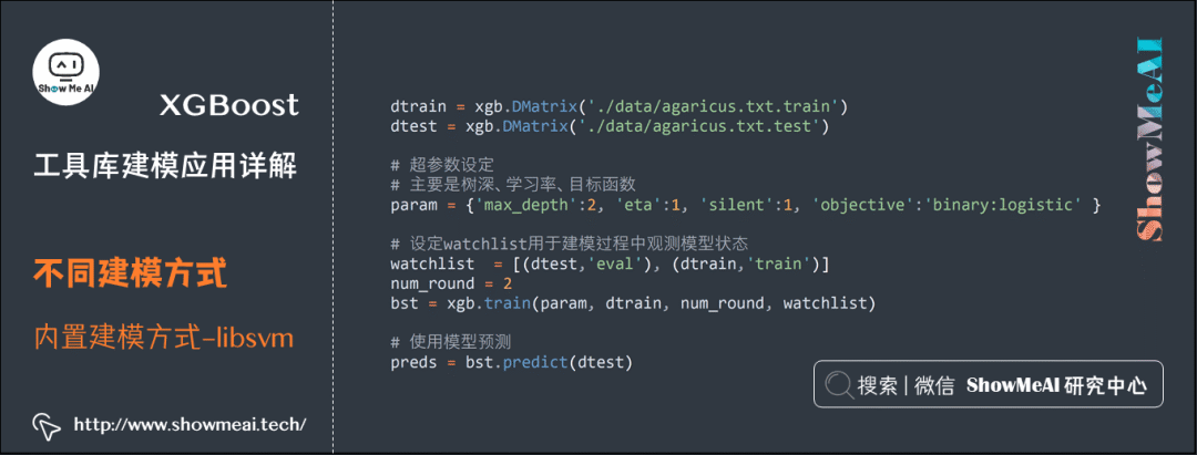

[0]  eval-error:0.042831  train-error:0.046522
[1]  eval-error:0.021726  train-error:0.022263
Error rate is 0.021726

Built-in Modeling Method: CSV Format Data Source

In the following example, the input data source is a csv file. We use the familiar Pandas toolkit (refer to ShowMeAI’s tutorial Data Analysis Series Tutorial^[4] and Data Science Tools Quick Reference | Pandas User Guide^[5]) to read the data into DataFrame format, then build the DMatrix format input, and subsequently use the built-in modeling method for training.

# Pima Indian Diabetes dataset includes many fields: number of pregnancies, plasma glucose concentration in oral glucose tolerance test, diastolic pressure (mm Hg), triceps skinfold thickness (mm),
# 2-hour serum insulin (μU/ml), body mass index (kg/(height(m)^2)), diabetes pedigree function, age (years)
import pandas as pd
data = pd.read_csv('./data/Pima-Indians-Diabetes.csv')
data.head()

# Import the toolkit
import numpy as np
import pandas as pd
import pickle
import xgboost as xgb
from sklearn.model_selection import train_test_split

# Read data using pandas
data = pd.read_csv('./data/Pima-Indians-Diabetes.csv')

# Split the data
train, test = train_test_split(data)

# Convert to DMatrix format
feature_columns = ['Pregnancies', 'Glucose', 'BloodPressure', 'SkinThickness', 'Insulin', 'BMI', 'DiabetesPedigreeFunction', 'Age']
target_column = 'Outcome'

# Extract numpy array values from DataFrame to initialize DMatrix object
xgtrain = xgb.DMatrix(train[feature_columns].values, train[target_column].values)
xgtest = xgb.DMatrix(test[feature_columns].values, test[target_column].values)

# Set parameters
param = {'max_depth':5, 'eta':0.1, 'silent':1, 'subsample':0.7, 'colsample_bytree':0.7, 'objective':'binary:logistic' }

# Set watchlist to observe model status
watchlist  = [(xgtest,'eval'), (xgtrain,'train')]
num_round = 10
bst = xgb.train(param, xgtrain, num_round, watchlist)

# Use the model for prediction
preds = bst.predict(xgtest)

# Calculate accuracy
labels = xgtest.get_label()
print('Error class is %f' % 
       (sum(1 for i in range(len(preds)) if int(preds[i]>0.5)!=labels[i]) /float(len(preds))))

# Save the model
bst.save_model('./model/0002.model')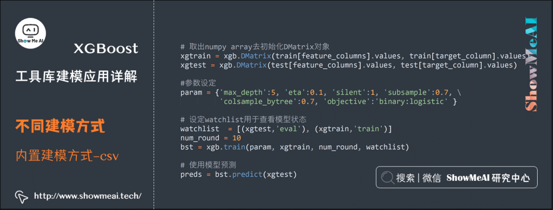

[0]  eval-error:0.354167  train-error:0.194444
[1]  eval-error:0.34375   train-error:0.170139
[2]  eval-error:0.322917  train-error:0.170139
[3]  eval-error:0.28125   train-error:0.161458
[4]  eval-error:0.302083  train-error:0.147569
[5]  eval-error:0.286458  train-error:0.138889
[6]  eval-error:0.296875  train-error:0.142361
[7]  eval-error:0.291667  train-error:0.144097
[8]  eval-error:0.302083  train-error:0.130208
[9]  eval-error:0.291667  train-error:0.130208
Error class is 0.291667

Estimator Modeling Method: SKLearn Interface + DataFrame

XGBoost also supports modeling using the unified estimator interface in SKLearn. Below is a typical reference case. For training and testing sets read as DataFrame format, you can directly use XGBoost to initialize XGBClassifier for fitting training. The usage and interface are consistent with other estimators in SKLearn.

# Import the toolkit
import numpy as np
import pandas as pd
import pickle
import xgboost as xgb
from sklearn.model_selection import train_test_split

# Read data using pandas
data = pd.read_csv('./data/Pima-Indians-Diabetes.csv')

# Split the data
train, test = train_test_split(data)

# Feature columns
feature_columns = ['Pregnancies', 'Glucose', 'BloodPressure', 'SkinThickness', 'Insulin', 'BMI', 'DiabetesPedigreeFunction', 'Age']
# Target column
target_column = 'Outcome'

# Initialize the model
xgb_classifier = xgb.XGBClassifier(n_estimators=20,\
                                   max_depth=4, \
                                   learning_rate=0.1, \
                                   subsample=0.7, \
                                   colsample_bytree=0.7, \
                                   eval_metric='error')

# Fit the model with DataFrame format data
xgb_classifier.fit(train[feature_columns], train[target_column])

# Use the model for prediction
preds = xgb_classifier.predict(test[feature_columns])

# Calculate accuracy
print('Error class is %f' %((preds!=test[target_column]).sum()/float(test_y.shape[0])))

# Save the model
joblib.dump(xgb_classifier, './model/0003.model')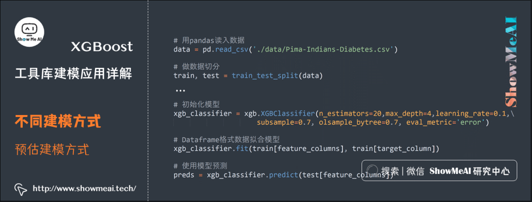

Error class is 0.265625

['./model/0003.model']

4. Model Tuning and Advanced Features

XGBoost Parameter Details

Before running XGBoost, three types of parameters must be set: General parameters, Booster parameters, and Task parameters:

General parameters:

This parameter controls which booster to use during the boosting process. Common boosters include tree models and linear models.

Booster parameters:

These depend on which booster is used and include parameters for the tree model booster and the linear booster.

Task parameters:

Controls the learning scenario. For example, different parameters are used for regression problems to control ranking.

(1) General Parameters

booster [default=gbtree]

There are two models to choose from: gbtree and gblinear. gbtree uses tree-based models for boosting calculations, while gblinear uses linear models. The default value is gbtree.

silent [default=0]

When set to 1, it indicates that runtime information will be printed; when set to 0, it indicates that it will run silently without printing runtime information. The default value is 0.

nthread

The number of threads used during XGBoost runtime. The default value is the maximum number of threads available on the current system.

num_pbuffer

Size of the prediction buffer, usually set to the number of training instances. The buffer is used to store the prediction results of the last boosting step and does not require manual setting.

num_feature

The number of feature dimensions used during boosting. This is set to the number of features. XGBoost will set it automatically and does not require manual setting.

(2) Tree Model Booster Parameters

eta [default=0.3]

To prevent overfitting, the shrinkage step length used in the update process. After each boosting calculation, the algorithm directly obtains the weights of new features.

eta makes the boosting calculation process more conservative by reducing the weights of features. The default value is 0.3, and the range is [0,1].

gamma [default=0]

The minimum loss reduction required for a tree to further split and grow. the larger, the more conservative the algorithm will be. The range is [0,∞).

max_depth [default=6]

The maximum depth of the tree. The default value is 6, and the range is [0,∞).

min_child_weight [default=1]

The minimum sum of sample weights in a child node. If the sum of sample weights in a leaf node is less than min_child_weight, the splitting process ends.

In current regression models, this parameter refers to the minimum number of samples required to build each model. The larger this parameter, the more conservative the algorithm. The range is [0,∞).

max_delta_step [default=0]

The maximum value allowed for weight estimation for each tree. If set to 0, it means no constraints; if set to a positive value, it can make the updates more conservative.

This parameter is usually unnecessary, but it may help in cases of extreme imbalance in logistic regression. Setting its range between 1-10 may control the updates. The range is [0,∞).

subsample [default=1]

The proportion of the subsample used to train the model from the entire sample set. If set to 0.5, it means XGBoost will randomly sample 50% from the entire sample set to build the tree model, which can prevent overfitting. The range is (0,1].

colsample_bytree [default=1]

The proportion of features sampled when building the tree. The default value is 1, and the range is (0,1].

(3) Linear Booster Parameters

lambda [default=0]

L2 regularization penalty coefficient.

alpha [default=0]

L1 regularization penalty coefficient.

lambda_bias

L2 regularization on bias. The default value is 0 (there is no regularization on bias in L1 because it is not important).

(4) Task Parameters

objective [default=reg:linear]

Defines the learning task and corresponding learning objectives.

Optional objective functions include:

base_score [default=0.5]

eval_metric [default according to objective]

The evaluation metric required for validation data. Different objective functions will have default evaluation metrics (rmse for regression, and error for classification, mean average precision for ranking).

Users can add multiple evaluation metrics. For Python users, parameters must be passed to the program as a list, rather than as a map, as list parameters will not override eval_metric.

Available options include:

seed [default=0]

Random number seed. The default value is 0.

Built-in Parameter Optimization

(1) Cross-Validation

XGBoost comes with some methods for experimentation and parameter tuning, including the cross-validation method xgb.cv.

xgb.cv(param, dtrain, num_round, nfold=5,metrics={'error'}, seed = 0)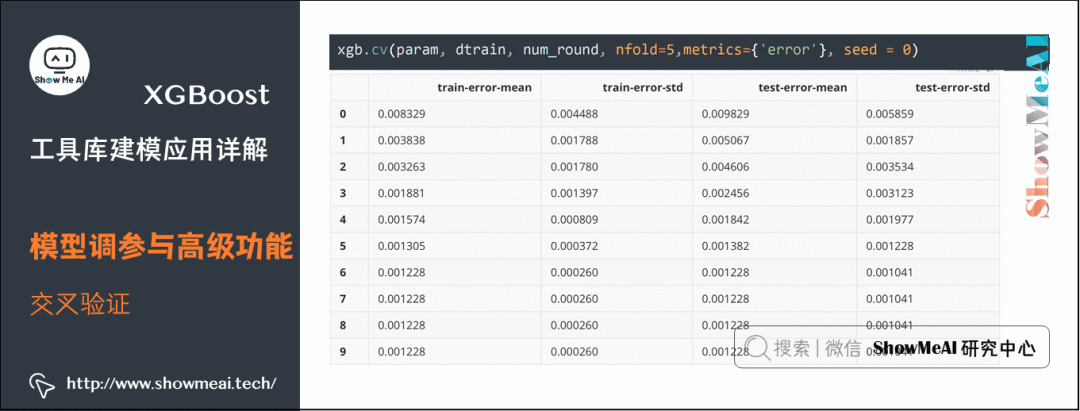

(2) Adding Preprocessing

We can add some settings during the data modeling process to the cross-validation phase, such as weighting different categories of samples. Below is a code example:

# Calculate the ratio of positive and negative samples, adjust sample weights
def fpreproc(dtrain, dtest, param):
    label = dtrain.get_label()
    ratio = float(np.sum(label == 0)) / np.sum(label==1)
    param['scale_pos_weight'] = ratio
    return (dtrain, dtest, param)

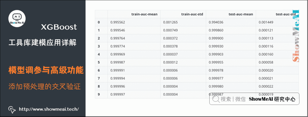
# Preprocess first, calculate sample weights, then do cross-validation
xgb.cv(param, dtrain, num_round, nfold=5,
       metrics={'auc'}, seed = 0, fpreproc = fpreproc)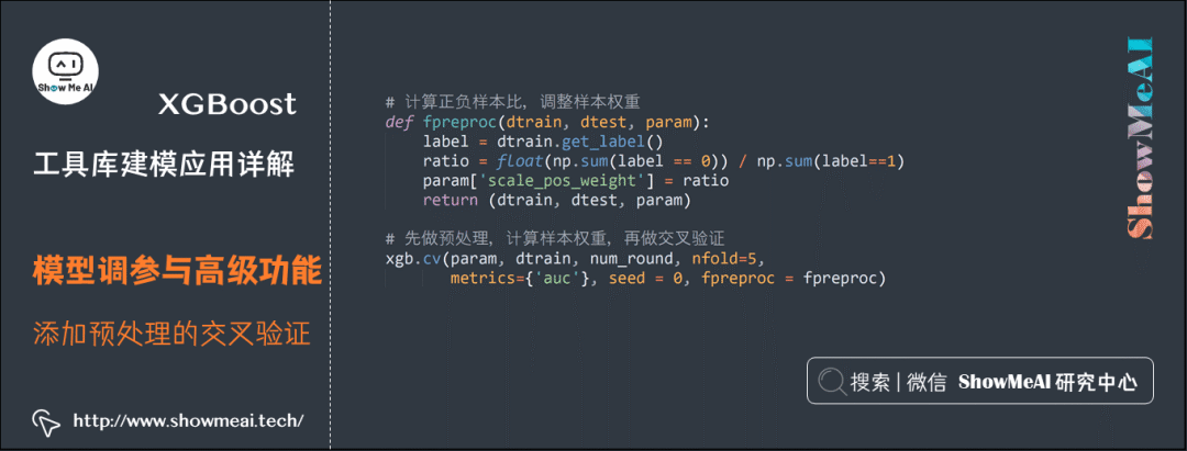

(3) Custom Loss Functions and Evaluation Criteria

XGBoost supports custom loss functions and evaluation criteria during training. The definition of the loss function needs to return the first and second derivatives of the loss function, while the evaluation criteria need to calculate the difference between the data’s label and the predicted values. The loss function is used for tree structure learning during the training process, while the evaluation criteria are often used for performance evaluation on the validation set.

print('Using custom loss function for cross-validation')
# Custom loss function, must provide the first and second derivatives of the loss function
def logregobj(preds, dtrain):
    labels = dtrain.get_label()
    preds = 1.0 / (1.0 + np.exp(-preds))
    grad = preds - labels
    hess = preds * (1.0-preds)
    return grad, hess

# Custom evaluation criteria, evaluate the gap between predicted values and the standard answers
def evalerror(preds, dtrain):
    labels = dtrain.get_label()
    return 'error', float(sum(labels != (preds > 0.0))) / len(labels)

watchlist  = [(dtest,'eval'), (dtrain,'train')]
param = {'max_depth':3, 'eta':0.1, 'silent':1}
num_round = 5
# Custom loss function training
bst = xgb.train(param, dtrain, num_round, watchlist, logregobj, evalerror)
# Cross-validation
xgb.cv(param, dtrain, num_round, nfold = 5, seed = 0, obj = logregobj, feval=evalerror)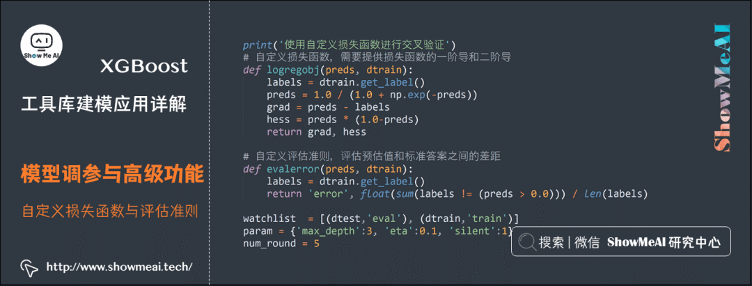

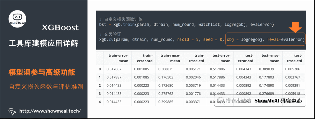
Using custom loss function for cross-validation
[0]  eval-rmse:0.306901   train-rmse:0.306164  eval-error:0.518312  train-error:0.517887
[1]  eval-rmse:0.179189   train-rmse:0.177278  eval-error:0.518312  train-error:0.517887
[2]  eval-rmse:0.172565   train-rmse:0.171728  eval-error:0.016139  train-error:0.014433
[3]  eval-rmse:0.269612   train-rmse:0.27111   eval-error:0.016139  train-error:0.014433
[4]  eval-rmse:0.396903   train-rmse:0.398256  eval-error:0.016139  train-error:0.014433

(4) Predicting Using Only the First n Trees

For boosting models, many base learners (often many trees in XGBoost) will be trained. We can train completely once and predict using only the ensemble of the first n trees.

#!/usr/bin/python
import numpy as np
import pandas as pd
import pickle
import xgboost as xgb
from sklearn.model_selection import train_test_split

# Basic example, read data from csv file, perform binary classification

# Read data using pandas
data = pd.read_csv('./data/Pima-Indians-Diabetes.csv')

# Split the data
train, test = train_test_split(data)

# Convert to DMatrix format
feature_columns = ['Pregnancies', 'Glucose', 'BloodPressure', 'SkinThickness', 'Insulin', 'BMI', 'DiabetesPedigreeFunction', 'Age']
target_column = 'Outcome'
xgtrain = xgb.DMatrix(train[feature_columns].values, train[target_column].values)
xgtest = xgb.DMatrix(test[feature_columns].values, test[target_column].values)

# Set parameters
param = {'max_depth':5, 'eta':0.1, 'silent':1, 'subsample':0.7, 'colsample_bytree':0.7, 'objective':'binary:logistic' }

# Set watchlist to observe model status
watchlist  = [(xgtest,'eval'), (xgtrain,'train')]
num_round = 10
bst = xgb.train(param, xgtrain, num_round, watchlist)

# Predict using only the first tree
ypred1 = bst.predict(xgtest, ntree_limit=1)
# Predict using the first 9 trees
ypred2 = bst.predict(xgtest, ntree_limit=9)
label = xgtest.get_label()
print('Error rate using the first tree is %f' % (np.sum((ypred1>0.5)!=label) /float(len(label))))
print('Error rate using the first 9 trees is %f' % (np.sum((ypred2>0.5)!=label) /float(len(label))))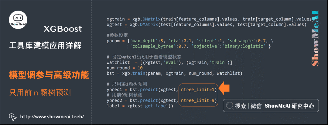

[0]  eval-error:0.255208  train-error:0.196181
[1]  eval-error:0.234375  train-error:0.175347
[2]  eval-error:0.25   train-error:0.163194
[3]  eval-error:0.229167  train-error:0.149306
[4]  eval-error:0.213542  train-error:0.154514
[5]  eval-error:0.21875   train-error:0.152778
[6]  eval-error:0.21875   train-error:0.154514
[7]  eval-error:0.213542  train-error:0.138889
[8]  eval-error:0.1875 train-error:0.147569
[9]  eval-error:0.1875 train-error:0.144097
Error rate using the first tree is 0.255208
Error rate using the first 9 trees is 0.187500

Estimator Tuning Optimization

(1) SKLearn Shape Interface Experiment Evaluation

XGBoost has an SKLearn estimator shape interface, and the overall usage is consistent with other estimators in SKLearn. Below is a manual cross-validation example. Note that here we directly use XGBClassifier for fitting and evaluating DataFrame data.

import pickle
import xgboost as xgb

import numpy as np
from sklearn.model_selection import KFold, train_test_split, GridSearchCV
from sklearn.metrics import confusion_matrix, mean_squared_error
from sklearn.datasets import load_iris, load_digits, load_boston

rng = np.random.RandomState(31337)

# Binary classification: confusion matrix
print("Binary classification problem for digits 0 and 1")
digits = load_digits(2)
y = digits['target']
X = digits['data']
# Data splitting object
kf = KFold(n_splits=2, shuffle=True, random_state=rng)
print("Cross-validation on 2 folds")
# 2-fold cross-validation
for train_index, test_index in kf.split(X):
    xgb_model = xgb.XGBClassifier().fit(X[train_index],y[train_index])
    predictions = xgb_model.predict(X[test_index])
    actuals = y[test_index]
    print("Confusion matrix:")
    print(confusion_matrix(actuals, predictions))

# Multiclass: confusion matrix
print("\nIris: Multiclass")
iris = load_iris()
y = iris['target']
X = iris['data']
kf = KFold(n_splits=2, shuffle=True, random_state=rng)
print("Cross-validation on 2 folds")
for train_index, test_index in kf.split(X):
    xgb_model = xgb.XGBClassifier().fit(X[train_index],y[train_index])
    predictions = xgb_model.predict(X[test_index])
    actuals = y[test_index]
    print("Confusion matrix:")
    print(confusion_matrix(actuals, predictions))

# Regression problem: MSE
print("\nBoston housing price regression prediction problem")
boston = load_boston()
y = boston['target']
X = boston['data']
kf = KFold(n_splits=2, shuffle=True, random_state=rng)
print("Cross-validation on 2 folds")
for train_index, test_index in kf.split(X):
    xgb_model = xgb.XGBRegressor().fit(X[train_index],y[train_index])
    predictions = xgb_model.predict(X[test_index])
    actuals = y[test_index]
    print("MSE:",mean_squared_error(actuals, predictions))

Binary classification problem for digits 0 and 1
Cross-validation on 2 folds
Confusion matrix:
[[87  0]
 [ 1 92]]
Confusion matrix:
[[91  0]
 [ 3 86]]

Iris: Multiclass
Cross-validation on 2 folds
Confusion matrix:
[[19  0  0]
 [ 0 31  3]
 [ 0  1 21]]
Confusion matrix:
[[31  0  0]
 [ 0 16  0]
 [ 0  3 25]]

Boston housing price regression prediction problem
Cross-validation on 2 folds
MSE: 9.860776812557337
MSE: 15.942418468446029

(2) Grid Search for Hyperparameter Tuning

As mentioned, the XGBoost estimator interface is consistent with other estimators in SKLearn, so we can also use hyperparameter tuning methods from SKLearn for model tuning.

Below is a typical example of grid search tuning hyperparameters, where we provide a candidate parameter list dictionary and perform cross-validation experiments using GridSearchCV to select the optimal hyperparameters for XGBoost from the candidates.

print("Parameter optimization:")
y = boston['target']
X = boston['data']
xgb_model = xgb.XGBRegressor()
clf = GridSearchCV(xgb_model,
                   {'max_depth': [2,4,6],
                    'n_estimators': [50,100,200]}, verbose=1)
clf.fit(X,y)
print(clf.best_score_)
print(clf.best_params_)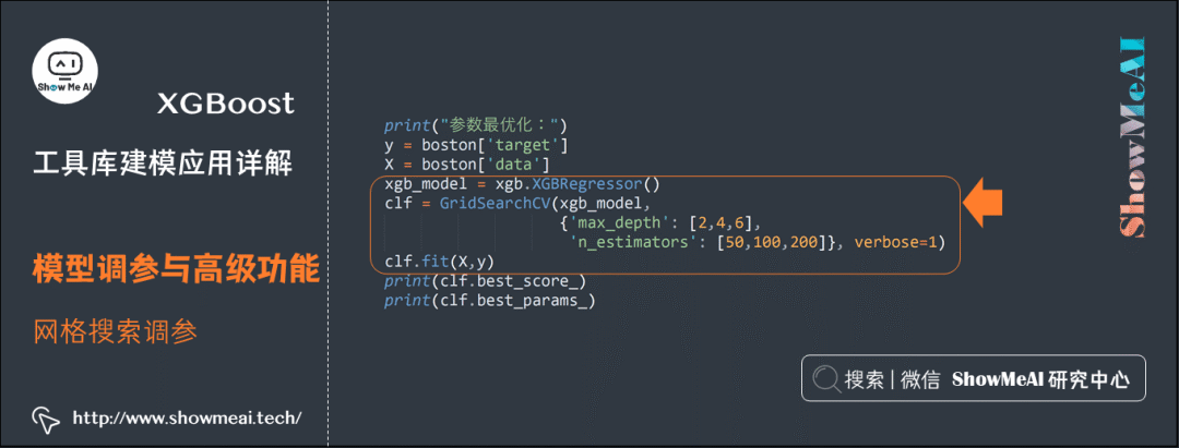

Parameter optimization:
Fitting 3 folds for each of 9 candidates, totalling 27 fits

[Parallel(n_jobs=1)]: Using backend SequentialBackend with 1 concurrent workers.

0.6001029721598573
{'max_depth': 4, 'n_estimators': 100}

[Parallel(n_jobs=1)]: Done  27 out of  27 | elapsed:    1.3s finished

(3) Early Stopping

XGBoost models can sometimes overfit the training set due to continuously adding new trees (correcting some samples that are not fitted correctly on the training set).

Early stopping is an effective strategy. The specific approach is to monitor the performance on the validation set during the process of continuously adding trees to the training set. If there is no improvement in the evaluation criteria for a certain number of rounds, it will revert to the best point on the validation set history and save it as the best model.

Below is the corresponding code example, where the parameter early_stopping_rounds sets the maximum number of rounds for which no improvement in performance on the validation set is acceptable, and eval_set specifies the validation dataset.

# Learn the model on the training set, adding one tree at a time, and monitor the effect on the validation set. When the effect on the validation set no longer improves, stop adding and growing trees.
X = digits['data']
y = digits['target']
X_train, X_val, y_train, y_val = train_test_split(X, y, random_state=0)
clf = xgb.XGBClassifier()
clf.fit(X_train, y_train, early_stopping_rounds=10, eval_metric="auc",
        eval_set=[(X_val, y_val)])

[0]  validation_0-auc:0.999497
Will train until validation_0-auc hasn't improved in 10 rounds.
[1]  validation_0-auc:0.999497
[2]  validation_0-auc:0.999497
[3]  validation_0-auc:0.999749
[4]  validation_0-auc:0.999749
[5]  validation_0-auc:0.999749
[6]  validation_0-auc:0.999749
[7]  validation_0-auc:0.999749
[8]  validation_0-auc:0.999749
[9]  validation_0-auc:0.999749
[10] validation_0-auc:1
[11] validation_0-auc:1
[12] validation_0-auc:1
[13] validation_0-auc:1
[14] validation_0-auc:1
[15] validation_0-auc:1
[16] validation_0-auc:1
[17] validation_0-auc:1
[18] validation_0-auc:1
[19] validation_0-auc:1
Stopping. Best iteration:
[10] validation_0-auc:1

(4) Feature Importance

During the XGBoost modeling process, you can also learn the corresponding feature importance information, which is stored in the model’s feature_importances_ attribute. Below is the code for visualizing feature importance:

iris = load_iris()
y = iris['target']
X = iris['data']
xgb_model = xgb.XGBClassifier().fit(X,y)

print('Feature ranking:')
feature_names=['sepal_length', 'sepal_width', 'petal_length', 'petal_width']
feature_importances = xgb_model.feature_importances_
indices = np.argsort(feature_importances)[::-1]

for index in indices:
    print("Feature %s importance is %f" %(feature_names[index], feature_importances[index]))

%matplotlib inline
import matplotlib.pyplot as plt
plt.figure(figsize=(16,8))
plt.title("Feature Importances")
plt.bar(range(len(feature_importances)), feature_importances[indices], color='b')
plt.xticks(range(len(feature_importances)), np.array(feature_names)[indices], color='b')

Feature ranking:
Feature petal_length importance is 0.415567
Feature petal_width importance is 0.291557
Feature sepal_length importance is 0.179420
Feature sepal_width importance is 0.113456

(5) Parallel Training Acceleration

In multi-resource scenarios, XGBoost can achieve parallel training acceleration. Below is an example code:

import os

if __name__ == "__main__":
    try:
        from multiprocessing import set_start_method
    except ImportError:
        raise ImportError("Unable to import multiprocessing.set_start_method."
                          " This example only runs on Python 3.4")
    #set_start_method("forkserver")

    import numpy as np
    from sklearn.model_selection import GridSearchCV
    from sklearn.datasets import load_boston
    import xgboost as xgb

    rng = np.random.RandomState(31337)

    print("Parallel Parameter optimization")
    boston = load_boston()

    os.environ["OMP_NUM_THREADS"] = "2"  # or to whatever you want
    y = boston['target']
    X = boston['data']
    xgb_model = xgb.XGBRegressor()
    clf = GridSearchCV(xgb_model, {'max_depth': [2, 4, 6],
                                   'n_estimators': [50, 100, 200]}, verbose=1,
                       n_jobs=2)
    clf.fit(X, y)
    print(clf.best_score_)
    print(clf.best_params_)

Parallel Parameter optimization
Fitting 3 folds for each of 9 candidates, totalling 27 fits

[Parallel(n_jobs=2)]: Using backend LokyBackend with 2 concurrent workers.
[Parallel(n_jobs=2)]: Done  24 out of  27 | elapsed:    2.2s remaining:    0.3s

0.6001029721598573
{'max_depth': 4, 'n_estimators': 100}

[Parallel(n_jobs=2)]: Done  27 out of  27 | elapsed:    2.4s finished

References