Bert is something that probably doesn’t need much introduction. Although I’m not a big fan of Bert, I must say it has indeed caused quite a stir in the NLP community. Nowadays, whether in Chinese or English, there is a plethora of popular science articles and interpretations about Bert, which seems to have surpassed the momentum of Word2Vec when it first came out. Interestingly, Bert was developed by Google, just like Word2Vec was. Regardless of which one you use, you are essentially following in the footsteps of Google’s big shots.

Shortly after Bert was released, some readers suggested that I write an interpretation, but I ultimately didn’t. On one hand, there are already many interpretations of Bert; on the other hand, Bert is essentially a large-scale pre-trained model based on Attention, which is not technically innovative. Moreover, I have already written an interpretation of Google’s Attention, so I didn’t feel motivated to write another one.

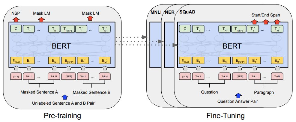
▲ Bert’s Pretraining and Fine-tuning (Image from Bert’s original paper)

Overall, I have never been particularly interested in Bert until I tried it for the first time at the end of last month while participating in an information extraction competition. After all, even if I wasn’t interested, I still had to learn it; using it and knowing how to use it are two different things. Additionally, there seems to be little documentation on using (fine-tuning) Bert in Keras, so I’d like to share my experience.

When Bert Meets Keras

Fortunately, there is already a well-packaged Keras version of Bert that allows for direct use of the officially released pre-trained weights. For readers who already have some Keras foundation, this might be the simplest way to call Bert. The phrase “standing on the shoulders of giants” perfectly describes our feelings as Keras enthusiasts at this moment.

keras-bert

I believe that the best packaging for Bert under Keras currently is:

keras-bert:

https://github.com/CyberZHG/keras-bert

This article is also based on it. By the way, besides keras-bert, CyberZHG has also packaged many valuable Keras modules, such as keras-gpt-2 (you can use the GPT2 model just like you use Bert), keras-lr-multiplier (layered learning rate settings), keras-ordered-neurons (which is the ON-LSTM introduced not long ago), etc. It seems that he is also a die-hard fan of Keras, hats off to him.

You can check the summary here:

https://github.com/CyberZHG/summary

In fact, with keras-bert, along with a little Keras foundational knowledge, and the demo provided by keras-bert being comprehensive enough, invoking and fine-tuning Bert has become a task with little technical content. Therefore, I will only provide a few Chinese examples to help readers get familiar with the basic usage of keras-bert.

Tokenizer

Before diving into the examples, it is necessary to discuss the Tokenizer related content. We import Bert’s Tokenizer and reconstruct it:

from keras_bert import load_trained_model_from_checkpoint, Tokenizer
import codecs


config_path = '../bert/chinese_L-12_H-768_A-12/bert_config.json'
checkpoint_path = '../bert/chinese_L-12_H-768_A-12/bert_model.ckpt'
dict_path = '../bert/chinese_L-12_H-768_A-12/vocab.txt'

token_dict = {}
with codecs.open(dict_path, 'r', 'utf8') as reader:
    for line in reader:
        token = line.strip()
        token_dict[token] = len(token_dict)

class OurTokenizer(Tokenizer):
    def _tokenize(self, text):
        R = []
        for c in text:
            if c in self._token_dict:
                R.append(c)
            elif self._is_space(c):
                R.append('[unused1]') # space类用未经训练的[unused1]表示
            else:
                R.append('[UNK]') # 剩余的字符是[UNK]
        return R

tokenizer = OurTokenizer(token_dict)
tokenizer.tokenize(u'今天天气不错')
# 输出是 ['[CLS]', u'今', u'天', u'天', u'气', u'不', u'错', '[SEP]']

Here is a brief explanation of the output result of the Tokenizer. First, by default, the beginning and end of the tokenized sentence will be marked with [CLS] and [SEP], respectively. The output vector corresponding to the [CLS] position represents the entire sentence vector (that’s how Bert is designed), while [SEP] serves as the separator between sentences, and the remaining parts are single-character outputs (for Chinese).

The Tokenizer originally has its own _tokenize method, which I have overridden here to ensure that the result after tokenization has the same length as the original string (if you count the two markers, then it is the same length plus 2). The built-in _tokenize of the Tokenizer will automatically remove spaces, and some characters will stick together in the output, resulting in the tokenized list not being equal to the original string’s length. This can be problematic for tasks like sequence labeling.

To avoid this hassle, I decided to rewrite it myself. The main idea is to use [unused1] to represent space characters, while other characters not in the list are represented by [UNK]. The [unused*] markers are untrained (randomly initialized) and are reserved by Bert for incrementally adding vocabulary, so we can use them to represent any new characters.

Three Examples

Here are three examples of keras-bert, namely text classification, relation extraction, and subject extraction, all fine-tuned based on the officially released pre-trained weights.

Bert Official Github:

https://github.com/google-research/bert

Official Chinese Pre-trained Weights:

https://storage.googleapis.com/bert_models/2018_11_03/chinese_L-12_H-768_A-12.zip

Examples Github:

https://github.com/bojone/bert_in_keras/

According to the official introduction, this weight was trained using Chinese Wikipedia as the corpus.

Text Classification

As the first example, we will do a basic text classification task. After getting familiar with this basic task, the remaining various tasks will become quite simple. This time, we will take the previously discussed sentiment classification task as an example, using the labeled data that was organized before.

Let’s take a look at the overall model; the complete code can be found at:

https://github.com/bojone/bert_in_keras/blob/master/sentiment.py

bert_model = load_trained_model_from_checkpoint(config_path, checkpoint_path)

for l in bert_model.layers:
    l.trainable = True

x1_in = Input(shape=(None,))
x2_in = Input(shape=(None,))

x = bert_model([x1_in, x2_in])
x = Lambda(lambda x: x[:, 0])(x) # 取出[CLS]对应的向量用来做分类
p = Dense(1, activation='sigmoid')(x)

model = Model([x1_in, x2_in], p)
model.compile(
    loss='binary_crossentropy',
    optimizer=Adam(1e-5), # 用足够小的学习率
    metrics=['accuracy']
)
model.summary()

Thus, invoking Bert in Keras for the sentiment classification task is complete.

Does it feel like the model code ended too soon? The Keras invocation of Bert is that concise. In fact, the only line that truly invokes Bert is load_trained_model_from_checkpoint; the rest are just ordinary Keras operations (thanks again to CyberZHG). Therefore, if you are already familiar with Keras, invoking Bert is a piece of cake.

With such a simple invocation, what accuracy can be achieved? After fine-tuning for 5 epochs, the best accuracy on the validation set was 95.5%+! Previously, in our article “Text Sentiment Classification (Part Three): Tokenization OR No Tokenization”, we only managed around 90% accuracy; after using Bert, with just a few lines of code, we improved accuracy by over 5 percentage points! It’s no wonder Bert has stirred up a wave in the NLP community.

Here, I would like to address two questions that readers might be concerned about based on my personal experience.

The first question, which many people might be interested in, is “How much GPU memory is enough?” In fact, there is no standard answer to this; the usage of GPU memory depends on three factors: sentence length, batch size, and model complexity. For instance, in the sentiment analysis example above, it can run on my GTX1060 with 6GB of memory, as long as the batch size is set to 24.

So if your GPU memory is not large enough, try reducing the maxlen of the sentences and the batch size. Of course, if your task is too complex, even a smaller maxlen and batch size might still result in OOM, and you would have to upgrade your GPU.

The second question is “What principles guide which layers should follow Bert?” The answer is: Use as few layers as possible to complete your task.

For example, the sentiment analysis above is just a binary classification task, so you can just take the first vector and add a Dense(1); don’t think about adding more Dense layers, and definitely don’t think about adding an LSTM followed by Dense; if you want to do sequence labeling (like NER), just add a Dense+CRF, and don’t add anything else.

In short, keep additional components to a minimum. One reason is that Bert itself is complex enough and has sufficient capability to handle many tasks you want to accomplish; another reason is that the layers you add are randomly initialized, and adding too many will cause severe disturbance to Bert’s pre-trained weights, which can reduce effectiveness or even cause the model not to converge.

Relation Extraction

If readers have a certain foundation in Keras, after learning the first example, we should have fully mastered Bert’s fine-tuning, as it is incredibly simple to explain. Therefore, the next two examples mainly provide reference patterns for readers to experience how to “use as few layers as possible to complete their tasks”.

In the second example, we introduce a minimalist relation extraction model based on Bert, whose annotation principle is similar to that described in “A Lightweight Information Extraction Model Based on DGCNN and Probabilistic Graph”; however, thanks to Bert’s powerful encoding capabilities, the portion we wrote can be greatly simplified.

In a reference implementation provided by me, the model part is as follows; see the complete model at:

https://github.com/bojone/bert_in_keras/blob/master/relation_extract.py

t = bert_model([t1, t2])
ps1 = Dense(1, activation='sigmoid')(t)
ps2 = Dense(1, activation='sigmoid')(t)

subject_model = Model([t1_in, t2_in], [ps1, ps2]) # 预测subject的模型


k1v = Lambda(seq_gather)([t, k1])
k2v = Lambda(seq_gather)([t, k2])
kv = Average()([k1v, k2v])
t = Add()([t, kv])
po1 = Dense(num_classes, activation='sigmoid')(t)
po2 = Dense(num_classes, activation='sigmoid')(t)

object_model = Model([t1_in, t2_in, k1_in, k2_in], [po1, po2]) # 输入text和subject，预测object及其关系

train_model = Model([t1_in, t2_in, s1_in, s2_in, k1_in, k2_in, o1_in, o2_in],
                    [ps1, ps2, po1, po2])

If you have read the article “A Lightweight Information Extraction Model Based on DGCNN and Probabilistic Graph”, you will understand how simple and clear the above implementation is compared to the model architecture without Bert.

We can see that we introduced Bert as an encoder, then obtained the encoded sequence t, and directly connected it to two Dense(1) layers to complete the subject labeling model; then, we took the corresponding encoding vectors of the input s and directly added them to the encoded vector sequence t, followed by two Dense(num_classes) layers to complete the object labeling model (while labeling the relationship).

How good can such a simple design achieve in terms of F1? The answer is: the offline dev can reach nearly 82%, and I submitted once online, resulting in 85%+ (all single models)!

In contrast, the model in “A Lightweight Information Extraction Model Based on DGCNN and Probabilistic Graph” needed to connect CNN, required global features, needed to pass s into LSTM for encoding, and required relative position vectors, with various improvised modules fused together, achieving only slightly better results (about 82.5%) with a single model.

It’s worth noting that I wrote this simple model based on Bert in just an hour, while the DGCNN model, which incorporates various techniques and models, took me nearly two months to debug!

Note: This model’s fine-tuning is best done with more than 8GB of GPU memory. Additionally, since I only started using Bert a few days before the competition ended, I wrote this model based on Bert without spending much time debugging, so the final submission result did not include Bert.

The example of using Bert for relation extraction has a notable difference from the previous sentiment analysis example regarding the learning rate. In the sentiment analysis example, a constant learning rate was used, and after training for several epochs, the results were quite good.

In the relation extraction example, the learning rate gradually increases from 0 during the first epoch to (this is called warmup), and during the second epoch, it decreases from to . In summary, the learning rate increases first and then decreases; Bert itself is trained using a similar learning rate curve, making this training method stable and less prone to failure while achieving better results.

Event Subject Extraction

The last example comes from CCKS 2019, focusing on event subject extraction in the financial field. This competition is still ongoing, but I have lost motivation and interest in continuing, so I am releasing my current model (accuracy of 89%+) for reference, wishing the participants who continue to compete better results.

Let’s briefly introduce the data for this competition:

Input:“Company A’s product had additives, and its subsidiary Company B and Company C were investigated”, “Product had issues”

Output:“Company A”

In other words, this is a dual-input, single-output model, where the input is a query and an event type, and the output is an entity (only one, and it is a fragment of the query). This task can actually be seen as a simplified version of SQUAD 1.0, and based on this output feature, it would be better to use a pointer structure (two softmaxes predicting the start and end).

The remaining question is: how to handle dual inputs?

Although the first two examples had different complexities, they were both single-input tasks; how do we handle dual inputs? Of course, since the entity types are limited, direct embedding is also feasible, but I opted for a simpler and more robust scheme that showcases Bert’s simplicity and power: directly concatenating the two inputs into one sentence, transforming it into a single input!

For example, the sample input above is processed as:

Input:“___Product had issues___Company A’s product had additives, and its subsidiary Company B and Company C were investigated”

Output:“Company A”

Now, it has transformed into a regular single-input extraction problem. Speaking of which, the code for this model is straightforward; please see:

https://github.com/bojone/bert_in_keras/blob/master/subject_extract.py

x = bert_model([x1, x2])
ps1 = Dense(1, use_bias=False)(x)
ps1 = Lambda(lambda x: x[0][..., 0] - (1 - x[1][..., 0]) * 1e10)([ps1, x_mask])
ps2 = Dense(1, use_bias=False)(x)
ps2 = Lambda(lambda x: x[0][..., 0] - (1 - x[1][..., 0]) * 1e10)([ps2, x_mask])

model = Model([x1_in, x2_in], [ps1, ps2])

Additionally, with some decoding tricks and model fusion, submitting this can achieve 89%+. When looking at the current leaderboard, I find that the best result is just over 90%, so it seems everyone is doing something similar.

This code shows considerable variability in results during repeated experiments, so I recommend running it multiple times to find the optimal result.

This example mainly tells us that when implementing your task with Bert, it’s best to organize it into a single-input format; this makes it simpler and more efficient.

For instance, when creating a sentence similarity model, where the input is two sentences and the output is a similarity score, there are two approaches: the first is to pass the two sentences through the same Bert and take the [CLS] features for classification; the second is to concatenate the two sentences into one, as described above, passing it through a single Bert, and then classifying the output features. The latter is evidently faster and allows for more comprehensive interaction between features.

Article Summary

This article introduces the basic invocation methods of Bert under Keras, primarily providing three reference examples for readers to gradually familiarize themselves with the fine-tuning steps and principles of Bert. Many of these are personal experiences from my own closed-door practice, and if there are any biases, I hope readers will point them out.

In fact, with the keras-bert implemented by CyberZHG, using Bert under Keras is a piece of cake, and after some tinkering, everyone can get the hang of it. Finally, I wish everyone a smooth experience!

Related Links

[1] https://kexue.fm/archives/3863

[2] https://kexue.fm/archives/3414

[3] https://kexue.fm/archives/6671

[4] https://biendata.com/competition/ccks_2019_4/

[5] https://rajpurkar.github.io/SQuAD-explorer/explore/1.1/dev/