

Author: Mirko Translated by: Sour Bun

Wishing you a peaceful Dragon Boat Festival
Generative Adversarial Network Applications in Quantitative Investing Series (Part 1)
Get the complete code at the end of the article
1
Introduction
Overfitting is one of the challenges we face when applying machine learning techniques to time series. This issue arises because we train our models using the only time series path we know: the realized history.
In particular, not all market mechanisms or events are well represented in our data. In fact, events that are very unlikely to occur, such as periods of extremely high volatility, are often underrepresented, which leads to poor model training. Thus, when these trained algorithms face new scenarios, they may fail; this can happen if we allow them to remain in production for too long without any precautions.
Now, what if we could train a model to generate new data for the same asset? What if we had a tool that could produce alternative actual time series with the same statistical properties as the original time series?? With such a tool, we could augment our training set with data from unlikely events or rare market mechanisms; thus, we would be able to build better generalized models, allowing practitioners to perform better simulations and trades, and backtests.Recently published authors in the Journal of Financial Data Science demonstrated how training deep models on synthetic data can reduce overfitting and improve performance.

It turns out that Generative Adversarial Networks (GANs) can do this.
Generative Adversarial Networks are a type of deep learning model and one of the most promising methods for unsupervised learning on complex distributions in recent years. The model produces fairly good outputs through the adversarial learning between (at least) two modules in the framework: the Generative Model and the Discriminative Model. In the original GAN theory, it is not required that G and D are both neural networks; they just need to be functions that can fit the corresponding generative and discriminative tasks. However, in practice, deep neural networks are generally used as G and D. A good GAN application requires a good training method; otherwise, it may lead to unsatisfactory outputs due to the flexibility of the neural network model.
2
What This Article Aims to Tell You
Our goal here is not to delve deeply into the theory of GANs (there is plenty of information available online), although our ultimate goal is to use one or more well-trained generators to simultaneously produce multiple time series, we choose to start from simple to gradually proceed. In this regard, we first examine whether GANs can learn the data generation process (DGP) of series.
3
Model
We first write a Pytorch dataset to produce different sine functions. The Pytorch dataset is a convenient utility that makes data loading easier and enhances code readability. Check it out here.
Get the complete code at the end of the article
from typing import Sequence
from torch.utils.data import Dataset
import numpy as np

class Sines(Dataset):

    def __init__(self, frequency_range: Sequence[float], amplitude_range: Sequence[float],
                 n_series: int = 200, datapoints: int = 100, seed: int = None):
        """
        Pytorch Dataset to produce sines.
        y = A * sin(B * x)
        :param frequency_range: range of A
        :param amplitude_range: range of B
        :param n_series: number of sines in your dataset
        :param datapoints: length of each sample
        :param seed: random seed
        """
        self.n_series = n_series
        self.datapoints = datapoints
        self.seed = seed
        self.frequency_range = frequency_range
        self.amplitude_range = amplitude_range
        self.dataset = self._generate_sines()

    def __len__(self):
        return self.datapoints

    def __getitem__(self, idx):
        return self.dataset[idx]

    def _generate_sines(self):
        if self.seed is not None:
            np.random.seed(self.seed)

        x = np.linspace(start=0, stop=2 * np.pi, num=self.datapoints)
        low_freq, up_freq = self.frequency_range[0], self.frequency_range[1]
        low_amp, up_amp = self.amplitude_range[0], self.amplitude_range[1]

        freq_vector = (up_freq - low_freq) * np.random.rand(self.n_series, 1) + low_freq
        ampl_vector = (up_amp - low_amp) * np.random.rand(self.n_series, 1) + low_amp

        return ampl_vector * np.sin(freq_vector * x)
Then we choose Wasserstein GAN (WGAN), as this particular class of models has a strong theoretical foundation and significantly improves training stability; moreover, the loss is related to the convergence of the generator and the quality of the samples, which is very useful because researchers do not need to frequently check the generated samples to understand whether the model is improving. Finally, WGANs are more robust to mode collapse and architectural changes than standard GANs.
Key Points
It is important to note that since Ian Goodfellow proposed GANs in 2014, there have been issues such as training difficulties, the loss of the generator and discriminator not indicating the training progress, and the lack of diversity in generated samples. Since then, many papers have attempted to address these issues, but with limited success. WGANs successfully achieve the following explosive points:
-
Thoroughly resolves the instability issues of GAN training, eliminating the need to carefully balance the training levels of the generator and discriminator;
-
Fundamentally addresses the issue of mode collapse, ensuring the diversity of generated samples;
-
Finally, there is a numerical value during training, like cross-entropy or accuracy, to indicate the training progress; the smaller this value, the better the GAN is trained, indicating higher quality images generated by the generator;
-
All these benefits can be achieved without a meticulously designed network architecture; even a simple multilayer fully connected network can accomplish this.
Be sure to check out these two papers:
https://arxiv.org/pdf/1701.04862.pdf

https://arxiv.org/pdf/1701.07875.pdf
4
How Do WGANs Differ from GANs?
The loss function in standard GANs quantifies the distance between the training and generated data distributions. In fact, GANs are based on the idea that as training progresses, the parameters of the model are gradually updated, and the distribution learned by G converges to the true data distribution. This convergence must be as smooth as possible, and it must be remembered that the manner in which this sequence of distributions converges depends on how we calculate the distance between each pair of distributions.
Now, WGANs and standard GANs differ in how they quantify this distance. Conventional GANs achieve this through the Jensen-Shannon divergence, while WGANs use Wasserstein distance, which has better properties. In particular, the Wasserstein metric is continuous and has good gradients everywhere, thus allowing distributions to converge more smoothly even when the supports of the true and generated distributions lie on non-overlapping low-dimensional manifolds.
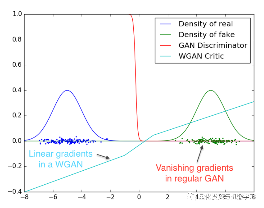
The above image shows how the discriminator in a standard GAN saturates, leading to gradient vanishing, while the discriminator in a WGAN provides very clear gradients across all parts of the space.
5
Lipschitz Constraint
The single Wasserstein distance is quite tricky; therefore, a clever trick is required: Kantorovich-Rubinstein duality—to overcome the obstacles and obtain the final form of our problem. Theoretically, the function f_w in the new form of Wasserstein metric must be K-Lipschitz continuous. f_w belongs to a sequence of parameterized functions; w represents a set of parameters, i.e., weights.
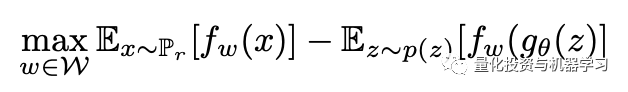
The final form of the objective function—the Wasserstein metric. The first expectation is calculated with respect to the true distribution, while the second expectation is calculated with respect to the noise distribution. z is the latent tensor, g_theta(z) represents the fake data generated by G. This objective function indicates that the critic is not directly attributed to probability. Instead, it is trained to learn a K-Lipschitz continuous function to help compute the final form of our Wasserstein distance.
We say a differentiable function is K-Lipschitz continuous if and only if it has a gradient with a norm at most K everywhere. k is called the Lipschitz constant.Lipschitz continuity is a promising technique for improving GAN training. Unfortunately, its implementation remains challenging. In fact, this is an active area of research, and there are several methods to strengthen the constraints. The original WGAN paper proposed weight clipping, but we adopted the “gradient penalty function” (GP) method because weight clipping can lead to capacity issues and requires additional parameters to define the space where the weights are located. On the other hand, the GP method can achieve more stable training with almost no hyperparameter tuning.
6
Architecture One
Our first architecture comes from this paper:
https://repository.tudelft.nl/islandora/object/uuid%3A51d69925-fb7b-4e82-9ba6-f8295f96705c
It proposes a WGAN-GP architecture to generate univariate synthetic financial time series. The proposed architecture is a mix of linear and convolutional layers in G and D, and it is ready to use. Unfortunately, despite the initial WGAN-GP paper clearly stating “no critic batch normalization”, training in this setup does not appear to be very stable, and batch normalization (BN) is used for D.
Thus, we removed BN and opted for spectral normalization. Simply put, SN ensures that D is K-Lipschitz continuous. To achieve this, it gradually applies to each layer of your critic to constrain its Lipschitz constant. Please refer to the following two articles for more details:
https://christiancosgrove.com/blog/2018/01/04/spectral-normalization-explained.html
https://arxiv.org/pdf/1802.05957.pdf
Although theoretically, with SN, we could remove the GP process term from the loss—signal-to-noise ratio and Gaussian processes should be considered as alternatives to enhance Lipschitz continuity—our tests do not support this proposition. However, SN improves training stability and accelerates convergence speed. Therefore, we use it in both G and D.
Finally, the original WGAN-GP paper suggested using the Adam optimizer in G and D, but we found that RMSprop better suits our needs based on experience.
Get the complete code at the end of the article
from torch import nn
from torch.nn.utils import spectral_norm

class AddDimension(nn.Module):
    def forward(self, x):
        return x.unsqueeze(1)


class SqueezeDimension(nn.Module):
    def forward(self, x):
        return x.squeeze(1)


def create_generator_architecture():
    return nn.Sequential(nn.Linear(50, 100),
                         nn.LeakyReLU(0.2, inplace=True),
                         AddDimension(),
                         spectral_norm(nn.Conv1d(1, 32, 3, padding=1), n_power_iterations=10),
                         nn.Upsample(200),

                         spectral_norm(nn.Conv1d(32, 32, 3, padding=1), n_power_iterations=10),
                         nn.LeakyReLU(0.2, inplace=True),
                         nn.Upsample(400),

                         spectral_norm(nn.Conv1d(32, 32, 3, padding=1), n_power_iterations=10),
                         nn.LeakyReLU(0.2, inplace=True),
                         nn.Upsample(800),

                         spectral_norm(nn.Conv1d(32, 1, 3, padding=1), n_power_iterations=10),
                         nn.LeakyReLU(0.2, inplace=True),

                         SqueezeDimension(),
                         nn.Linear(800, 100)
                         )


def create_critic_architecture():
    return nn.Sequential(AddDimension(),
                         spectral_norm(nn.Conv1d(1, 32, 3, padding=1), n_power_iterations=10),
                         nn.LeakyReLU(0.2, inplace=True),
                         nn.MaxPool1d(2),

                         spectral_norm(nn.Conv1d(32, 32, 3, padding=1), n_power_iterations=10),
                         nn.LeakyReLU(0.2, inplace=True),
                         nn.MaxPool1d(2),

                         spectral_norm(nn.Conv1d(32, 32, 3, padding=1), n_power_iterations=10),
                         nn.LeakyReLU(0.2, inplace=True),
                         nn.Flatten(),

                         nn.Linear(800, 50),
                         nn.LeakyReLU(0.2, inplace=True),

                         nn.Linear(50, 15),
                         nn.LeakyReLU(0.2, inplace=True),

                         nn.Linear(15, 1)
                         )


class Generator(nn.Module):
    def __init__(self):
        super().__init__()
        self.main = create_generator_architecture()

    def forward(self, input):
        return self.main(input)


class Critic(nn.Module):
    def __init__(self):
        super().__init__()
        self.main = create_critic_architecture()

    def forward(self, input):
        return self.main(input)
To try it out, you will also need some code to compute the loss, backpropagate, update model weights, save logs, train samples, etc.:
import argparse
import os
import torch
from tqdm import tqdm
from torch.autograd import Variable
from torch.autograd import grad as torch_grad
import matplotlib.pyplot as plt
from torch.utils.tensorboard import writer, SummaryWriter
from torch.utils.data import DataLoader
from math import pi
from datasets.datasets import Sines
from models.wgangp import Generator, Critic

class Trainer:
    NOISE_LENGTH = 50

    def __init__(self, generator, critic, gen_optimizer, critic_optimizer,
                 gp_weight=10, critic_iterations=5, print_every=200, use_cuda=False, checkpoint_frequency=200):
        self.g = generator
        self.g_opt = gen_optimizer
        self.c = critic
        self.c_opt = critic_optimizer
        self.losses = {'g': [], 'c': [], 'GP': [], 'gradient_norm': []}
        self.num_steps = 0
        self.use_cuda = use_cuda
        self.gp_weight = gp_weight
        self.critic_iterations = critic_iterations
        self.print_every = print_every
        self.checkpoint_frequency = checkpoint_frequency

        if self.use_cuda:
            self.g.cuda()
            self.c.cuda()

    def _critic_train_iteration(self, real_data):

        batch_size = real_data.size()[0]
        noise_shape = (batch_size, self.NOISE_LENGTH)
        generated_data = self.sample_generator(noise_shape)

        real_data = Variable(real_data)

        if self.use_cuda:
            real_data = real_data.cuda()

        # Pass data through the Critic
        c_real = self.c(real_data)
        c_generated = self.c(generated_data)

        # Get gradient penalty
        gradient_penalty = self._gradient_penalty(real_data, generated_data)
        self.losses['GP'].append(gradient_penalty.data.item())

        # Create total loss and optimize
        self.c_opt.zero_grad()
        d_loss = c_generated.mean() - c_real.mean() + gradient_penalty
        d_loss.backward()
        self.c_opt.step()

        self.losses['c'].append(d_loss.data.item())

    def _generator_train_iteration(self, data):
        self.g_opt.zero_grad()
        batch_size = data.size()[0]
        latent_shape = (batch_size, self.NOISE_LENGTH)

        generated_data = self.sample_generator(latent_shape)

        # Calculate loss and optimize
        d_generated = self.c(generated_data)
        g_loss = - d_generated.mean()
        g_loss.backward()
        self.g_opt.step()
        self.losses['g'].append(g_loss.data.item())

    def _gradient_penalty(self, real_data, generated_data):

        batch_size = real_data.size()[0]

        # Calculate interpolation
        alpha = torch.rand(batch_size, 1)
        alpha = alpha.expand_as(real_data)
        if self.use_cuda:
            alpha = alpha.cuda()
        interpolated = alpha * real_data.data + (1 - alpha) * generated_data.data
        interpolated = Variable(interpolated, requires_grad=True)
        if self.use_cuda:
            interpolated = interpolated.cuda()

        # Pass interpolated data through Critic
        prob_interpolated = self.c(interpolated)

        # Calculate gradients of probabilities with respect to examples
        gradients = torch_grad(outputs=prob_interpolated, inputs=interpolated,
                               grad_outputs=torch.ones(prob_interpolated.size()).cuda() if self.use_cuda
                               else torch.ones(prob_interpolated.size()), create_graph=True,
                               retain_graph=True)[0]
        # Gradients have shape (batch_size, num_channels, series length),
        # here we flatten to take the norm per example for every batch
        gradients = gradients.view(batch_size, -1)
        self.losses['gradient_norm'].append(gradients.norm(2, dim=1).mean().data.item())

        # Derivatives of the gradient close to 0 can cause problems because of the
        # square root, so manually calculate norm and add epsilon
        gradients_norm = torch.sqrt(torch.sum(gradients ** 2, dim=1) + 1e-12)

        # Return gradient penalty
        return self.gp_weight * ((gradients_norm - 1) ** 2).mean()

    def _train_epoch(self, data_loader, epoch):
        for i, data in enumerate(data_loader):
            self.num_steps += 1
            self._critic_train_iteration(data.float())
            # Only update generator every critic_iterations iterations
            if self.num_steps % self.critic_iterations == 0:
                self._generator_train_iteration(data)

            if i % self.print_every == 0:
                global_step = i + epoch * len(data_loader.dataset)
                writer.add_scalar('Losses/Critic', self.losses['c'][-1], global_step)
                writer.add_scalar('Losses/Gradient Penalty', self.losses['GP'][-1], global_step)
                writer.add_scalar('Gradient Norm', self.losses['gradient_norm'][-1], global_step)

                if self.num_steps > self.critic_iterations:
                    writer.add_scalar('Losses/Generator', self.losses['g'][-1], global_step)

    def train(self, data_loader, epochs, plot_training_samples=True, checkpoint=None):

        if checkpoint:
            path = os.path.join('checkpoints', checkpoint)
            state_dicts = torch.load(path, map_location=torch.device('cpu'))
            self.g.load_state_dict(state_dicts['g_state_dict'])
            self.c.load_state_dict(state_dicts['d_state_dict'])
            self.g_opt.load_state_dict(state_dicts['g_opt_state_dict'])
            self.c_opt.load_state_dict(state_dicts['d_opt_state_dict'])

        if plot_training_samples:
            # Fix latents to see how series generation improves during training
            noise_shape = (1, self.NOISE_LENGTH)
            fixed_latents = Variable(self.sample_latent(noise_shape))
            if self.use_cuda:
                fixed_latents = fixed_latents.cuda()

        for epoch in tqdm(range(epochs)):

            # Sample a different region of the latent distribution to check for mode collapse
            dynamic_latents = Variable(self.sample_latent(noise_shape))
            if self.use_cuda:
                dynamic_latents = dynamic_latents.cuda()

            self._train_epoch(data_loader, epoch + 1)

            # Save checkpoint
            if epoch % self.checkpoint_frequency == 0:
                torch.save({
                    'epoch': epoch,
                    'd_state_dict': self.c.state_dict(),
                    'g_state_dict': self.g.state_dict(),
                    'd_opt_state_dict': self.c_opt.state_dict(),
                    'g_opt_state_dict': self.g_opt.state_dict(),
                }, 'checkpoints/epoch_{}.pkl'.format(epoch))

            if plot_training_samples and (epoch % self.print_every == 0):
                self.g.eval()
                # Generate fake data using both fixed and dynamic latents
                fake_data_fixed_latents = self.g(fixed_latents).cpu().data
                fake_data_dynamic_latents = self.g(dynamic_latents).cpu().data

                plt.figure()
                plt.plot(fake_data_fixed_latents.numpy()[0].T)
                plt.savefig('training_samples/fixed_latents/series_epoch_{}.png'.format(epoch))
                plt.close()

                plt.figure()
                plt.plot(fake_data_dynamic_latents.numpy()[0].T)
                plt.savefig('training_samples/dynamic_latents/series_epoch_{}.png'.format(epoch))
                plt.close()
                self.g.train()

    def sample_generator(self, latent_shape):
        latent_samples = Variable(self.sample_latent(latent_shape))
        if self.use_cuda:
            latent_samples = latent_samples.cuda()

        return self.g(latent_samples)

    @staticmethod
    def sample_latent(shape):
        return torch.randn(shape)

    def sample(self, num_samples):
        generated_data = self.sample_generator(num_samples)
        return generated_data.data.cpu().numpy()


if __name__ == '__main__':
    parser = argparse.ArgumentParser(prog='GANetano', usage='%(prog)s [options]')
    parser.add_argument('-ln', '--logname', type=str, dest='log_name', default=None, required=True,
                        help='tensorboard filename')
    parser.add_argument('-e', '--epochs', type=int, dest='epochs', default=15000, help='number of training epochs')
    parser.add_argument('-bs', '--batches', type=int, dest='batches', default=16,
                        help='number of batches per training iteration')
    parser.add_argument('-cp', '--checkpoint', type=str, dest='checkpoint', default=None,
                        help='checkpoint to use for a warm start')


    args = parser.parse_args()

    # Instantiate Generator and Critic + initialize weights
    g = Generator()

    g_opt = torch.optim.RMSprop(g.parameters(), lr=0.00005)
    d = Critic()

    d_opt = torch.optim.RMSprop(d.parameters(), lr=0.00005)

    # Create Dataloader
    dataset = Sines(frequency_range=[0, 2 * pi], amplitude_range=[0, 2 * pi], seed=42, n_series=200)
    dataloader = DataLoader(dataset, batch_size=args.batches)

    # Instantiate Trainer
    trainer = Trainer(g, d, g_opt, d_opt, use_cuda=torch.cuda.is_available())
    # Train model
    print('Training is about to start...')
    # Instantiate Tensorboard writer
    tb_logdir = os.path.join('..', 'tensorboard', args.log_name)
    writer = SummaryWriter(log_dir=tb_logdir)

    trainer.train(dataloader, epochs=args.epochs, plot_training_samples=True, checkpoint=args.checkpoint)
In order to test, you will also need a piece of code to compute the loss, backpropagate, update model weights, save logs, train samples, etc.:
import argparse
import os
import torch
from tqdm import tqdm
from torch.autograd import Variable
from torch.autograd import grad as torch_grad
import matplotlib.pyplot as plt
from torch.utils.tensorboard import writer, SummaryWriter
from torch.utils.data import DataLoader
from math import pi
from datasets.datasets import Sines
from models.wgangp import Generator, Critic

class Trainer:
    NOISE_LENGTH = 50

    def __init__(self, generator, critic, gen_optimizer, critic_optimizer,
                 gp_weight=10, critic_iterations=5, print_every=200, use_cuda=False, checkpoint_frequency=200):
        self.g = generator
        self.g_opt = gen_optimizer
        self.c = critic
        self.c_opt = critic_optimizer
        self.losses = {'g': [], 'c': [], 'GP': [], 'gradient_norm': []}
        self.num_steps = 0
        self.use_cuda = use_cuda
        self.gp_weight = gp_weight
        self.critic_iterations = critic_iterations
        self.print_every = print_every
        self.checkpoint_frequency = checkpoint_frequency

        if self.use_cuda:
            self.g.cuda()
            self.c.cuda()

    def _critic_train_iteration(self, real_data):

        batch_size = real_data.size()[0]
        noise_shape = (batch_size, self.NOISE_LENGTH)
        generated_data = self.sample_generator(noise_shape)

        real_data = Variable(real_data)

        if self.use_cuda:
            real_data = real_data.cuda()

        # Pass data through the Critic
        c_real = self.c(real_data)
        c_generated = self.c(generated_data)

        # Get gradient penalty
        gradient_penalty = self._gradient_penalty(real_data, generated_data)
        self.losses['GP'].append(gradient_penalty.data.item())

        # Create total loss and optimize
        self.c_opt.zero_grad()
        d_loss = c_generated.mean() - c_real.mean() + gradient_penalty
        d_loss.backward()
        self.c_opt.step()

        self.losses['c'].append(d_loss.data.item())

    def _generator_train_iteration(self, data):
        self.g_opt.zero_grad()
        batch_size = data.size()[0]
        latent_shape = (batch_size, self.NOISE_LENGTH)

        generated_data = self.sample_generator(latent_shape)

        # Calculate loss and optimize
        d_generated = self.c(generated_data)
        g_loss = - d_generated.mean()
        g_loss.backward()
        self.g_opt.step()
        self.losses['g'].append(g_loss.data.item())

    def _gradient_penalty(self, real_data, generated_data):

        batch_size = real_data.size()[0]

        # Calculate interpolation
        alpha = torch.rand(batch_size, 1)
        alpha = alpha.expand_as(real_data)
        if self.use_cuda:
            alpha = alpha.cuda()
        interpolated = alpha * real_data.data + (1 - alpha) * generated_data.data
        interpolated = Variable(interpolated, requires_grad=True)
        if self.use_cuda:
            interpolated = interpolated.cuda()

        # Pass interpolated data through Critic
        prob_interpolated = self.c(interpolated)

        # Calculate gradients of probabilities with respect to examples
        gradients = torch_grad(outputs=prob_interpolated, inputs=interpolated,
                               grad_outputs=torch.ones(prob_interpolated.size()).cuda() if self.use_cuda
                               else torch.ones(prob_interpolated.size()), create_graph=True,
                               retain_graph=True)[0]
        # Gradients have shape (batch_size, num_channels, series length),
        # here we flatten to take the norm per example for every batch
        gradients = gradients.view(batch_size, -1)
        self.losses['gradient_norm'].append(gradients.norm(2, dim=1).mean().data.item())

        # Derivatives of the gradient close to 0 can cause problems because of the
        # square root, so manually calculate norm and add epsilon
        gradients_norm = torch.sqrt(torch.sum(gradients ** 2, dim=1) + 1e-12)

        # Return gradient penalty
        return self.gp_weight * ((gradients_norm - 1) ** 2).mean()

    def _train_epoch(self, data_loader, epoch):
        for i, data in enumerate(data_loader):
            self.num_steps += 1
            self._critic_train_iteration(data.float())
            # Only update generator every critic_iterations iterations
            if self.num_steps % self.critic_iterations == 0:
                self._generator_train_iteration(data)

            if i % self.print_every == 0:
                global_step = i + epoch * len(data_loader.dataset)
                writer.add_scalar('Losses/Critic', self.losses['c'][-1], global_step)
                writer.add_scalar('Losses/Gradient Penalty', self.losses['GP'][-1], global_step)
                writer.add_scalar('Gradient Norm', self.losses['gradient_norm'][-1], global_step)

                if self.num_steps > self.critic_iterations:
                    writer.add_scalar('Losses/Generator', self.losses['g'][-1], global_step)

    def train(self, data_loader, epochs, plot_training_samples=True, checkpoint=None):

        if checkpoint:
            path = os.path.join('checkpoints', checkpoint)
            state_dicts = torch.load(path, map_location=torch.device('cpu'))
            self.g.load_state_dict(state_dicts['g_state_dict'])
            self.c.load_state_dict(state_dicts['d_state_dict'])
            self.g_opt.load_state_dict(state_dicts['g_opt_state_dict'])
            self.c_opt.load_state_dict(state_dicts['d_opt_state_dict'])

        if plot_training_samples:
            # Fix latents to see how series generation improves during training
            noise_shape = (1, self.NOISE_LENGTH)
            fixed_latents = Variable(self.sample_latent(noise_shape))
            if self.use_cuda:
                fixed_latents = fixed_latents.cuda()

        for epoch in tqdm(range(epochs)):

            # Sample a different region of the latent distribution to check for mode collapse
            dynamic_latents = Variable(self.sample_latent(noise_shape))
            if self.use_cuda:
                dynamic_latents = dynamic_latents.cuda()

            self._train_epoch(data_loader, epoch + 1)

            # Save checkpoint
            if epoch % self.checkpoint_frequency == 0:
                torch.save({
                    'epoch': epoch,
                    'd_state_dict': self.c.state_dict(),
                    'g_state_dict': self.g.state_dict(),
                    'd_opt_state_dict': self.c_opt.state_dict(),
                    'g_opt_state_dict': self.g_opt.state_dict(),
                }, 'checkpoints/epoch_{}.pkl'.format(epoch))

            if plot_training_samples and (epoch % self.print_every == 0):
                self.g.eval()
                # Generate fake data using both fixed and dynamic latents
                fake_data_fixed_latents = self.g(fixed_latents).cpu().data
                fake_data_dynamic_latents = self.g(dynamic_latents).cpu().data

                plt.figure()
                plt.plot(fake_data_fixed_latents.numpy()[0].T)
                plt.savefig('training_samples/fixed_latents/series_epoch_{}.png'.format(epoch))
                plt.close()

                plt.figure()
                plt.plot(fake_data_dynamic_latents.numpy()[0].T)
                plt.savefig('training_samples/dynamic_latents/series_epoch_{}.png'.format(epoch))
                plt.close()
                self.g.train()

    def sample_generator(self, latent_shape):
        latent_samples = Variable(self.sample_latent(latent_shape))
        if self.use_cuda:
            latent_samples = latent_samples.cuda()

        return self.g(latent_samples)

    @staticmethod
    def sample_latent(shape):
        return torch.randn(shape)

    def sample(self, num_samples):
        generated_data = self.sample_generator(num_samples)
        return generated_data.data.cpu().numpy()


if __name__ == '__main__':
    parser = argparse.ArgumentParser(prog='GANetano', usage='%(prog)s [options]')
    parser.add_argument('-ln', '--logname', type=str, dest='log_name', default=None, required=True,
                        help='tensorboard filename')
    parser.add_argument('-e', '--epochs', type=int, dest='epochs', default=15000, help='number of training epochs')
    parser.add_argument('-bs', '--batches', type=int, dest='batches', default=16,
                        help='number of batches per training iteration')
    parser.add_argument('-cp', '--checkpoint', type=str, dest='checkpoint', default=None,
                        help='checkpoint to use for a warm start')


    args = parser.parse_args()

    # Instantiate Generator and Critic + initialize weights
    g = Generator()

    g_opt = torch.optim.RMSprop(g.parameters(), lr=0.00005)
    d = Critic()

    d_opt = torch.optim.RMSprop(d.parameters(), lr=0.00005)

    # Create Dataloader
    dataset = Sines(frequency_range=[0, 2 * pi], amplitude_range=[0, 2 * pi], seed=42, n_series=200)
    dataloader = DataLoader(dataset, batch_size=args.batches)

    # Instantiate Trainer
    trainer = Trainer(g, d, g_opt, d_opt, use_cuda=torch.cuda.is_available())
    # Train model
    print('Training is about to start...')
    # Instantiate Tensorboard writer
    tb_logdir = os.path.join('..', 'tensorboard', args.log_name)
    writer = SummaryWriter(log_dir=tb_logdir)

    trainer.train(dataloader, epochs=args.epochs, plot_training_samples=True, checkpoint=args.checkpoint)
7
Results
The good news is that our model learned to generate realistic sine samples; the bad news is that sine waves are not asset returns! So, what is the next step to increase our trust in this model?
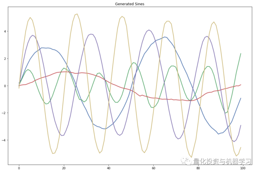
Using the trained model to generate different real sine waves
Why don’t we replace the simple sine function with samples from an ARMA process whose parameters we know to fill the GAN?
We chose a simple ARMA(1,1) process with p=0.7 and q=0.2, generated real samples with a new Pytorch dataset, and trained the model.
Get the complete code at the end of the article
class ARMA(Dataset):

    def __init__(self, p: Sequence[float], q: Sequence[float], seed: int = None,
                 n_series: int = 200, datapoints: int = 100):
        """
        Pytorch Dataset to sample a given ARMA process.

        y = ARMA(p,q)
        :param p: AR parameters
        :param q: MA parameters
        :param seed: random seed
        :param n_series: number of ARMA samples in your dataset
        :param datapoints: length of each sample
        """
        self.p = p
        self.q = q
        self.n_series = n_series
        self.datapoints = datapoints
        self.seed = seed
        self.dataset = self._generate_ARMA()

    def __len__(self):
        return self.datapoints

    def __getitem__(self, idx):
        return self.dataset[idx]

    def _generate_ARMA(self):

        if self.seed is not None:
            np.random.seed(self.seed)

        ar = np.array(self.p)
        ma = np.array(self.q)
        ar = np.r_[1, -ar]
        ma = np.r_[1, ma]
        burn = int(self.datapoints / 10)

        dataset = []

        for i in range(self.n_series):
            arma = smt.arma_generate_sample(ar=ar, ma=ma, nsample=self.datapoints, burnin=burn)
            dataset.append(arma)

        return np.array(dataset)
We now generate one hundred fake samples, estimate p and q, and see the results below. p and q are the only parameters of our DGP.
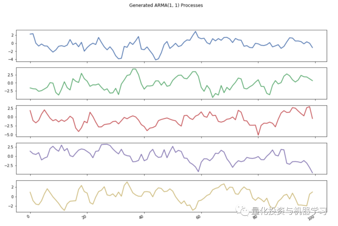
Synthetic ARMA(1,1) samples generated by the trained model
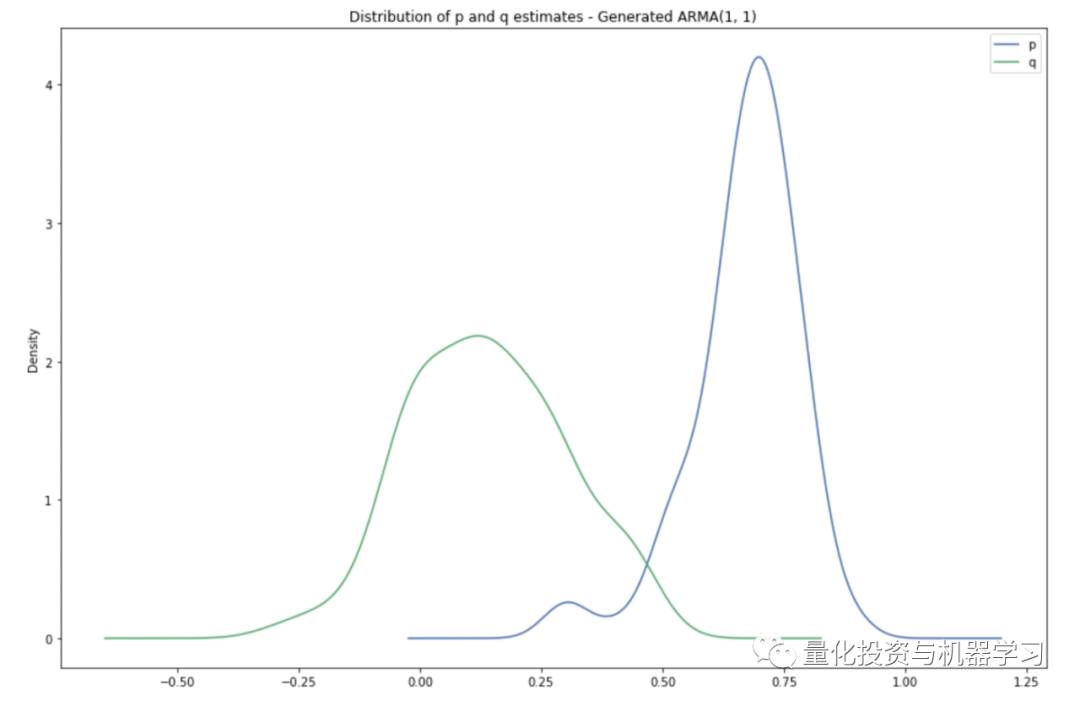
It can be seen that this model has learned the DGP well. In fact, the patterns of these distributions closely match the true parameters of the DGP, p and q, which are 0.7 and 0.2 respectively.
8
What Should the Loss Look Like?
In our first experiment, we constantly asked ourselves what we would get from our losses. Of course, it all depends on the training data you choose, the optimization algorithm, and the learning rate, but we have found that a successful training is characterized by a loss that, although initially unstable, gradually converges to lower values. Under the same conditions, reducing the learning rate can stabilize training.
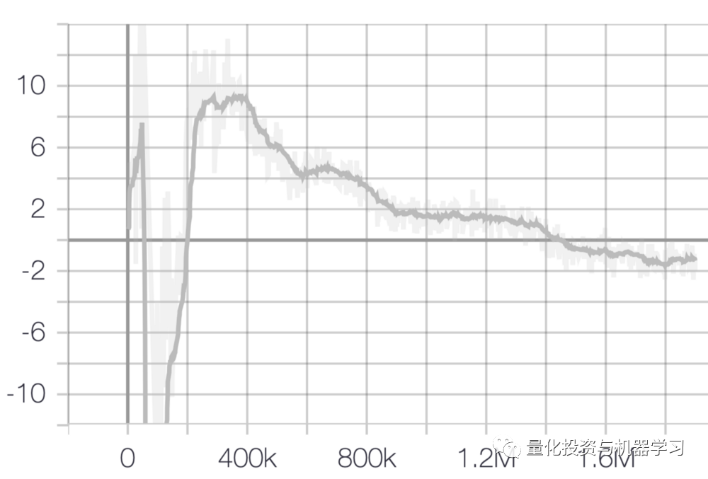
Example of generator loss
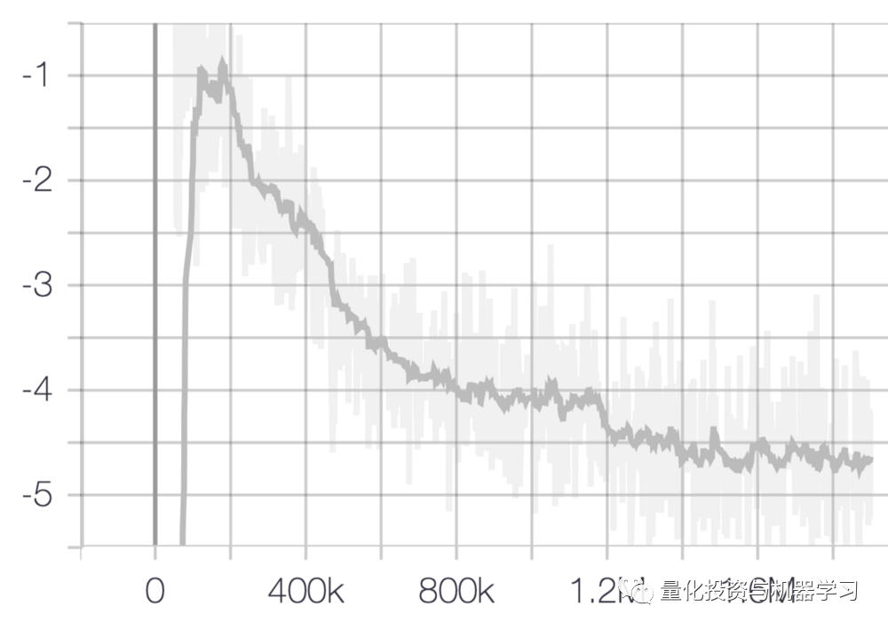
Example of critic loss
How to Check for Mode Collapse?
To check for mode collapse, we generate fake samples during training using different latent tensors each time. Through this process, we can see what happens when sampling from different parts of the noise space. If you sample with different random tensors and G continues to produce the same series, then you are experiencing mode collapse.
Key Points
Mode collapse refers to the phenomenon where the samples generated by GAN are homogeneous, believing that the results that meet a certain distribution are true while others are false, leading to the above results.
Natural data distributions are very complex and multimodal. That is, the data distribution has many peaks or modes. Each mode represents a cluster of similar data samples, but is different from other modes.
During mode collapse, the generative network G generates samples belonging to a limited set of modes. When G believes it can deceive the discriminator D on a single mode, G will generate samples outside that mode. This cycle continues indefinitely, limiting the diversity of generated samples.

The above image shows that GAN’s output does not exhibit mode collapse. The lower image shows mode collapse.
The discriminator will ultimately determine that the samples from that mode are fake. Eventually, the generative network G will simply lock onto another mode. This loop will continue indefinitely, limiting the diversity of generated samples.
Do GANs Provide Advantages Over Other Generative Mechanisms?
This is an important question, and we want to answer it through further experiments: the complexity of GANs must be demonstrated through better performance.
GP Constraint
According to this paper:
https://arxiv.org/pdf/1904.01184.pdf
The standard GP method may not be the best implementation of Lipschitz regularization. Moreover, spectral normalization may unnecessarily constrain the critic and weaken its ability to provide sound gradients to G. The authors propose an alternative method that can be used when the standard method fails. In subsequent articles in this series, we will validate their recommendations.
Why Should We Train D More Than G?
A well-trained D is crucial in the WGAN environment because the critic estimates the Wasserstein distance between the real and fake distributions. An optimal critic will provide a good estimate of our distance metric, which in turn will lead to healthy gradients!
9
Code Access
Backend Response
WGAN-1
We welcome everyone to continue to follow the subsequent articles in this series…
References
[2019] Towards Efficient and Unbiased Implementation of Lipschitz Continuity in GANs — Zhou, Shen et al
[2019] Enriching Financial Datasets with Generative Adversarial Networks, de Meer Pardo
[2018] Spectral Normalization for Generative Adversarial Networks — Miyato, Kataoka et al
[2017] Improved Training of Wasserstein GANs — Gulrajani, Ahmed et al
[2017] Wasserstein GAN — Arjovsky, Chintala et al
Quantitative Investment and Machine Learning WeChat Official Account is a mainstream self-media in the industry vertical to Quant, MFE, Fintech, AI, ML and other fields. The official account has more than 180,000 followers from various circles including public offerings, private equity, securities firms, futures, banks, insurance asset management, and overseas. It publishes cutting-edge research results and the latest quantitative information daily.
